Running a Simulation

Aim

To simulate a Dynamic TOPMODEL of the Eden catchment, visualise the output showing how the show how the parameters may be altered.

Required R packages

This exercise builds upon the early model creation, using the outputs generated during that exercise.

The packages used can be attached with

library("dynatop")
library("terra")
library("xts")

and remember to move to the eden_data directory e.g.

setwd("./eden_data")

A Simulation

The minimum data need to perform a simulation with dynatop is a model, such as that output by dynatopGIS in the previous section and observed data in the format introduced earlier.

Load the previously created data

mdl <- readRDS(file.path(".","dyna","atb_20_model.rds"))
output_defn <- readRDS(file.path(".","dyna","gauge_output_defn.rds"))
obs <- readRDS(file.path(".","processed","obs.rds"))

A dynatop object is initialised by loading the model

hru <- mdl$hru
ctch_mdl <- dynatop$new(hru)

This step performs some basic checks on the model for consistency. The data can then be added; again simple checks are performed.

ctch_mdl$add_data(obs)

The initial states of the HRUs can be specified in the model object. If, as in the case of this example, the states are not specified then any attempt to perform a simulation will fail.

## expect a failure
ctch_mdl$sim(output_defn)
#> Error in ctch_mdl$sim(output_defn): Model states have non-finite values

The states need to be initialised using the initialise method. This presumes:

• The surface is dry
• The root zone is partially full (the s_rz0 parameter)
• There is a specified (see below) recharge rate representing the flow from the unsaturated to saturated zone
• the saturated zone is at a steady state
• the unsaturated zone storage ensures that the recharge rate from the unsaturated zone to the saturated zone is as close to the maximum as possible

The maximum recharge rate and fraction of root zone storage full for each HRU forms part of its definition.

hru[[1000]]$initialisation
#>    s_rz_0 r_uz_sz_0 
#>   7.5e-01   1.0e-07
## s_rz_0 - fraction of root zone full
## r_us_sz_0 - recharge unsaturated to saturated zone in m/s and

A simple way of getting an initial estimate of the recharge is to divide the observed discharge at the outlet of the catchment for the first time step by the catchment area. This works best if the first time step has no rainfall and is close to base-flow.

## determining the initial recharge rate ad setting it in the model
r0 <- as.numeric(obs$Sheepmount_obs[1]) / sum( sapply( hru, function(x){x$properties["area"]} ) )
hru <- lapply(hru,function(h){h$initialisation["r_uz_sz_0"] <- r0;h})

In the following we initialise the states and then perform the simulation, using the chaining of commands.

## the map input is only needed for visualisation
ctch_mdl <- dynatop$new(hru,map=mdl$map)$add_data(obs)$initialise()$sim(output_defn)

Mass balance

It is possible to output the mass balance for each time step of the simulation using the get_mass_errors method. The returns an xts object giving the volumes in the hill-slope states at the start and end of the time step along with the other fluxes as volumes. This can easily be used to plot the errors as shown below.

mb <- ctch_mdl$get_mass_errors()
head(mb)
#>                     initial_state         p e_t  outflow final_state
#> 2020-02-01 00:15:00    -198322986  636.1126   0 170462.6  -198492812
#> 2020-02-01 00:30:00    -198492812  636.1126   0 170455.0  -198662631
#> 2020-02-01 00:45:00    -198662631 6385.7957   0 170447.6  -198826693
#> 2020-02-01 01:00:00    -198826693 6385.7957   0 170440.0  -198990747
#> 2020-02-01 01:15:00    -198990747 2140.9939   0 170432.2  -199159038
#> 2020-02-01 01:30:00    -199159038 2140.9939   0 170423.9  -199327321
#>                             error
#> 2020-02-01 00:15:00 -6.854534e-07
#> 2020-02-01 00:30:00  7.748604e-07
#> 2020-02-01 00:45:00  2.980232e-08
#> 2020-02-01 01:00:00 -1.400709e-06
#> 2020-02-01 01:15:00  3.278255e-07
#> 2020-02-01 01:30:00 -5.960464e-08
plot( mb$err , main="Mass balance error",ylab="m^3")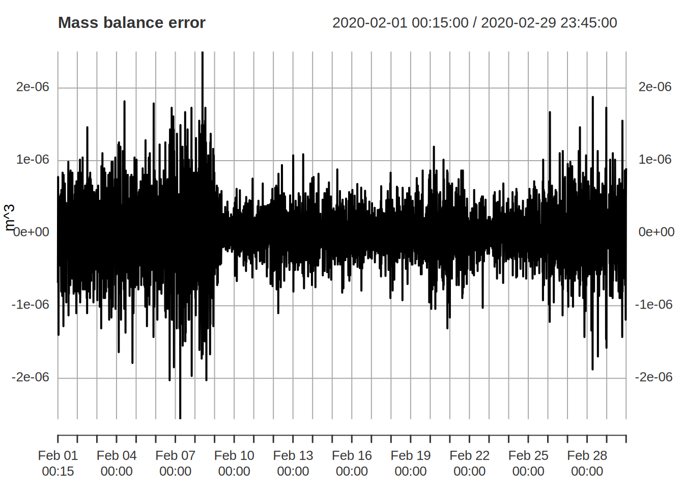

Visualisations

After a simulation it is possible to get or plot output. Two types of output are available:

• the time series variable specified in the output_defn used in the simulation
• the states of the system at end of the simulation

Both have methods for plotting the data or returning in as a variable as shown in the following

Gauge flows

## For simulated flows at the gauge sites
sim_gauge <- ctch_mdl$get_output() ## extract the flow as an xts object
head(sim_gauge)
#>                     Bampton Grange Burnbanks Coal Burn Cummersdale Dacre Bridge
#> 2020-02-01 00:15:00       4.928123  2.817783 0.1227015    21.63214     2.836557
#> 2020-02-01 00:30:00       4.926602  2.820096 0.1197231    21.62889     2.836551
#> 2020-02-01 00:45:00       4.925192  2.818703 0.1173275    21.62742     2.834431
#> 2020-02-01 01:00:00       4.922987  2.815001 0.1156495    21.62710     2.830495
#> 2020-02-01 01:15:00       4.919994  2.810062 0.1145420    21.62684     2.825530
#> 2020-02-01 01:30:00       4.916647  2.804287 0.1138176    21.62577     2.820491
#>                     Eamont Bridge Great Corby Greenholme Harraby Green
#> 2020-02-01 00:15:00      12.89632    110.4597   27.29113      14.33129
#> 2020-02-01 00:30:00      12.89247    110.4585   27.28848      14.32870
#> 2020-02-01 00:45:00      12.88853    110.4571   27.28491      14.32500
#> 2020-02-01 01:00:00      12.88497    110.4544   27.28030      14.32131
#> 2020-02-01 01:15:00      12.88187    110.4509   27.27486      14.31959
#> 2020-02-01 01:30:00      12.87922    110.4471   27.26884      14.32002
#>                     Hynam Bridge Kirkby Stephen Newbiggin Bridge
#> 2020-02-01 00:15:00     3.547355       5.248447         13.54109
#> 2020-02-01 00:30:00     3.546882       5.245908         13.54321
#> 2020-02-01 00:45:00     3.544828       5.242319         13.54446
#> 2020-02-01 01:00:00     3.541144       5.238129         13.54532
#> 2020-02-01 01:15:00     3.536149       5.233599         13.54379
#> 2020-02-01 01:30:00     3.530388       5.228567         13.53925
#>                     Pooley Bridge Upstream Sheepmount Stockdalewath
#> 2020-02-01 00:15:00               12.22210   188.7329      5.477744
#> 2020-02-01 00:30:00               12.22039   188.7357      5.475740
#> 2020-02-01 00:45:00               12.21934   188.7366      5.471281
#> 2020-02-01 01:00:00               12.21803   188.7354      5.466385
#> 2020-02-01 01:15:00               12.21524   188.7327      5.462073
#> 2020-02-01 01:30:00               12.21039   188.7281      5.458081
#>                     Temple Sowerby   Udford
#> 2020-02-01 00:15:00       47.70087 32.90629
#> 2020-02-01 00:30:00       47.69905 32.90238
#> 2020-02-01 00:45:00       47.69883 32.89939
#> 2020-02-01 01:00:00       47.69882 32.89724
#> 2020-02-01 01:15:00       47.69792 32.89562
#> 2020-02-01 01:30:00       47.69570 32.89389

## Plot the simulated flows at the gauges
ctch_mdl$plot_output()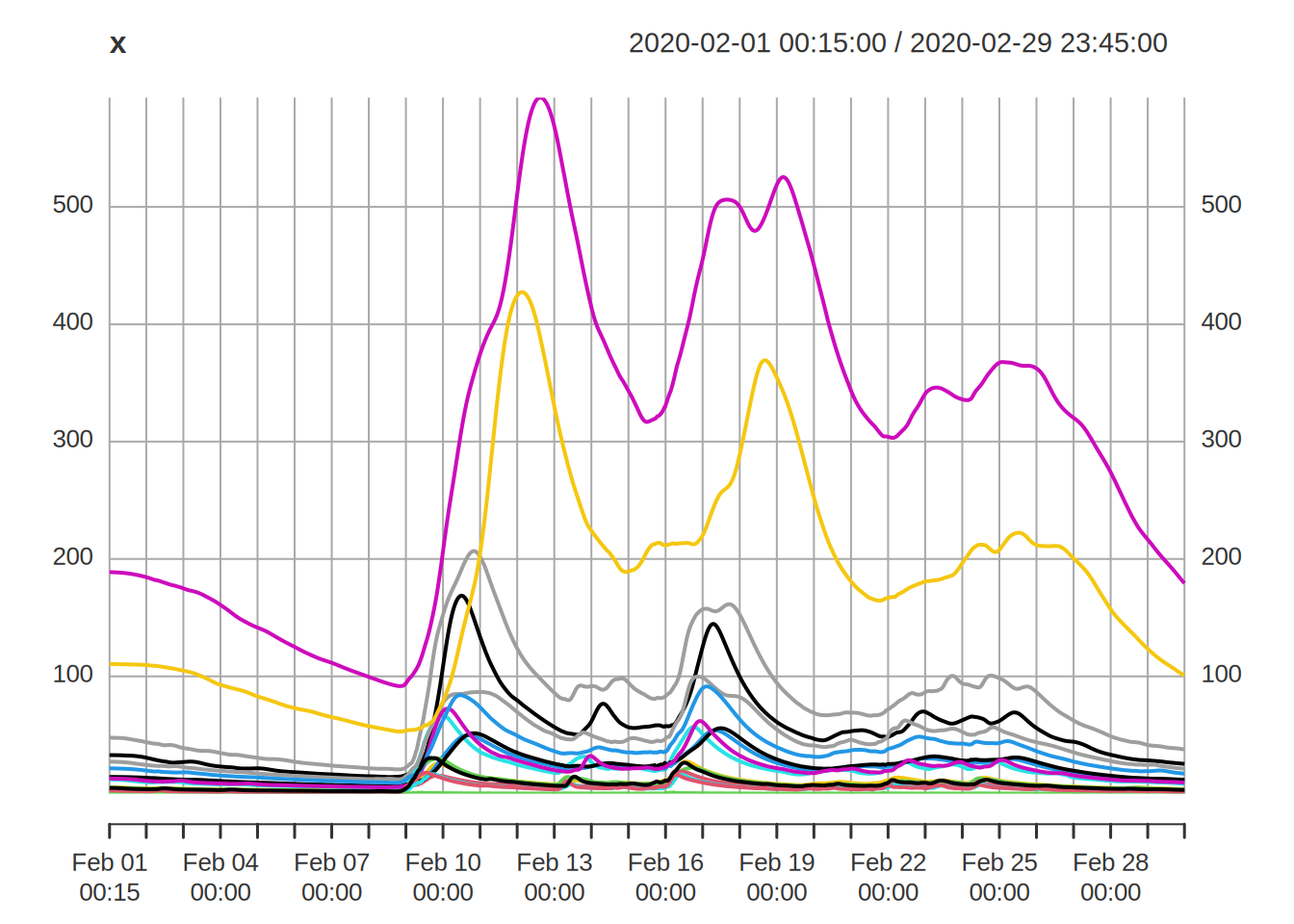

The observed gauge data is readily added and plotted

plot( merge(obs$Sheepmount_obs,sim_gauge),main="Simulated and observed flows",
     legend.loc='topright')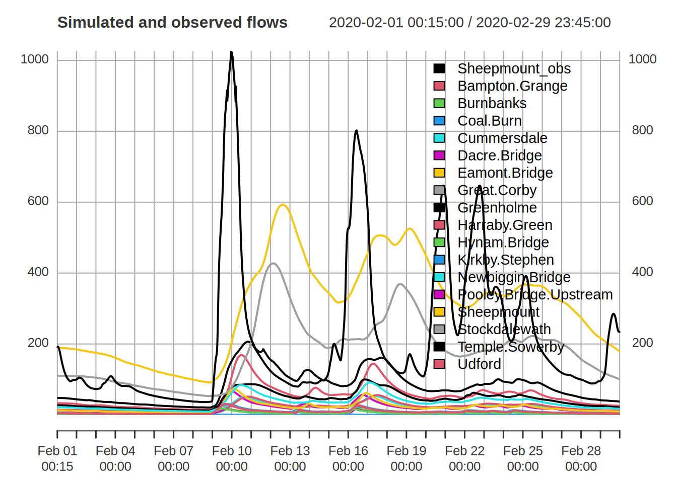

Current States

The current states of the model can be extracted and plotted.

## extract the current states as a data.frame
current_state <- ctch_mdl$get_states()
## columns correspond to the Hill-slope HRU ID, and the storage's in each of the four zones
head(current_state)
#>   id         s_sf s_rz s_uz s_sz
#> 1  0 0.0002079108  0.1    0    0
#> 2  1 9.9896233896  0.1    0    0
#> 3  2 0.0004973038  0.1    0    0
#> 4  3 0.0036077856  0.1    0    0
#> 5  4 0.0036269050  0.1    0    0
#> 6  5 0.5555132189  0.1    0    0

## a single state can be plotted at one time
ctch_mdl$plot_state("s_sz")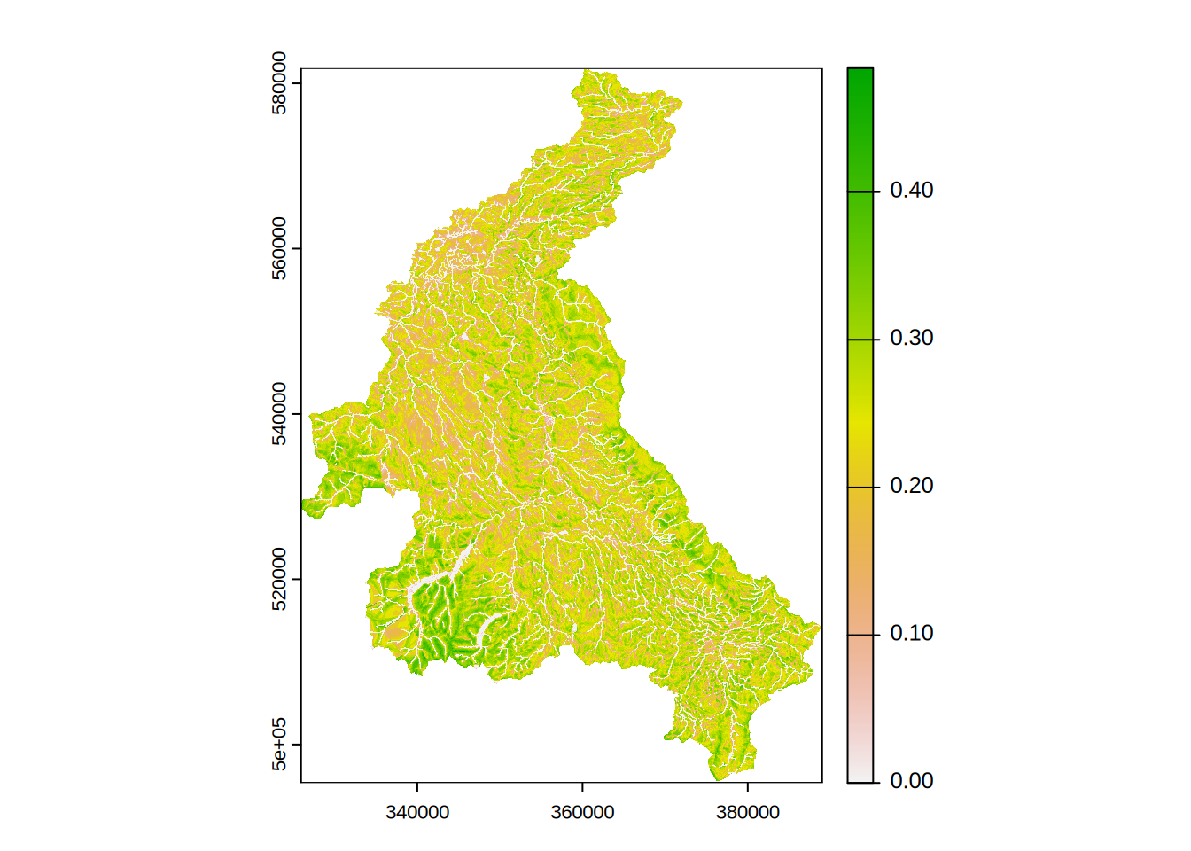

Changing Parameters

The parameters are stored within the HRU descriptions; particularly the sf, rz, uz and sz elements. Each of these contains a type variable and corresponding named vector of parameters. The various types and parameters for each zone are described in the (dynatop vignettes)[https://waternumbers.github.io/dynatop/articles/HRU.html#surface-zone-representations].

The most straight forward way for altering the parameters is two write a function that acts on each HRU, altering the parameters with reference to the properties of the HRU. The following presents a simple function of setting a faster surface velocity and kinematic solution for the river channels.

fpar <- function(h){ ## h is the hru
    ## test if a channel
    if( !is.na(h$class$startNode) ){
        ## change type
        h$sf$type <- "kin"
        h$sf$param["c_sf"] <- 1
    }
    h
}

Channel Inflow

To use dyantop to drive a hydraulic model the inflow from the subsurface and hillslope HRUs to the surface zone of each channel HRU may need to be computed. The first term is (directly available )[https://waternumbers.github.io/dynatop/articles/The_Model_Object.html#output_flux], though will the wrong sign and as a volume. Start by working out the id of each channel HRU

chn_id <- do.call(c, lapply( hru, function(h){ if(!is.na(h$class$startNode)){ h$id } }))

Next start creating an output definition for the flux from root zone

out_hyd <-  data.frame( name = paste0("hyd_",chn_id),
                       id = chn_id,
                       flux = "v_sf_rz", scale =-1/900) # scale is negative since flux usually downwards, 1/900 is 1/timestep

Next we will construct the inflow from HRUs representing hillslopes and add these to the data frame above.

## function to compute the relevent part so the output definition for each potential source HRU
fout <- function(h){
    ## test if it is a channel HRU - in which case return NULL
    if( !is.na(h$class$startNode) ){ return(NULL) }
        
    ## index of flow directiuons going to other channels
    idx <- h$sf_flow_direction$id %in% chn_id
    if(!any(idx)){ return(NULL) } ## quit if no links!
    ## create partial output defn
    data.frame(
        name = paste0("hyd_",h$sf_flow_direction$id[idx]), ## which inflow does it alter
        id = h$id, ## flux comes from this HRU
        flux = "q_sf", # surface flux out of this HRU is input to the next
        scale = h$sf_flow_direction$fraction[idx] # scale is fraction of flow (since taking it away)
    )
}
## row bind to give a data.frame
tmp <- do.call( rbind, lapply( hru, fout) )

## row bind onto the intial data frame
out_hyd <- rbind( out_hyd, tmp )

## sort this, not needed but easier to look at
out_hyd <- out_hyd[ order(out_hyd$name), ]

In the resulting output definition multiple fluxes contribute to the same output series, combined by a summation weighted by the scale value. Simulation and visualisation work as before.

ctch_mdl <- dynatop$new(hru)$add_data(obs)$initialise()$sim(out_hyd)
plot( ctch_mdl$get_output()[,1:10])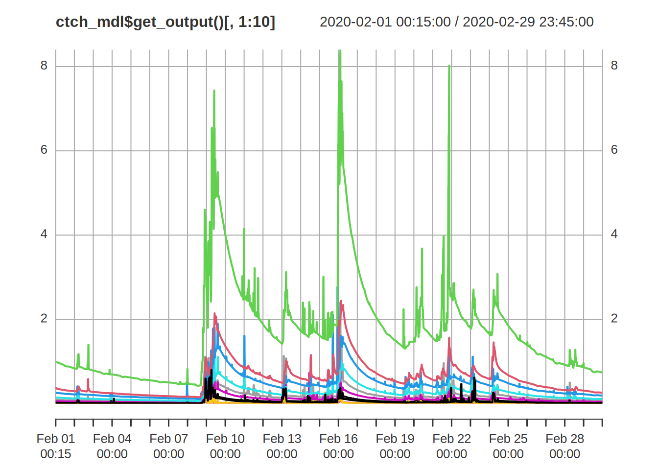

Extracting Intermediate States

Unless requested dynatop keeps only the final state during a simulation. To request that states are other time steps are kept a vector of times must be passed in the call to the sim method.

## Let us repeat the same simulation
## keeping the states for every other time step
keep_times <- index(obs)[seq(2,nrow(obs),by=96)] ## an vector of time steps
ctch_mdl$initialise()$sim(output_defn,keep_states=keep_times) ## passing the vector of time steps to the call

The record of the states can know be extracted. While there is an entry for every time step only those request will be populated

## extract the record of the states at each time step
state_rec <- ctch_mdl$get_states(record=TRUE) ## returns the whole record of states
head(names(state_rec)) ## the elements in state_rec are named after the time
#> [1] "2020-02-01 00:15:00" "2020-02-01 00:30:00" "2020-02-01 00:45:00"
#> [4] "2020-02-01 01:00:00" "2020-02-01 01:15:00" "2020-02-01 01:30:00"
head(sapply(state_rec,length)) ## those in keep_times are populated the remainder are empty
#> 2020-02-01 00:15:00 2020-02-01 00:30:00 2020-02-01 00:45:00 2020-02-01 01:00:00 
#>                   0                5322                   0                   0 
#> 2020-02-01 01:15:00 2020-02-01 01:30:00 
#>                   0                   0

The visualisation of the state record is possible either as a time series

## Create a time series plot of the saturated zone deficit
s_sz_rec <- state_rec[ sapply(state_rec,length)>0 ]
s_sz_rec <- lapply(s_sz_rec, function(x){ setNames( sapply(x,function(z){z$states["s_sz"]}), sapply(x,function(z){z$id}) )} )
s_sz_rec <- do.call(rbind,s_sz_rec) ## bind to make matrix
s_sz_rec <- as.xts(s_sz_rec) ## convert to and xts object using the rownames as times
## for a the Hill-slope HRUs with IDs 2487, 3598 and 5201 the start of the time series are
head(s_sz_rec[,c("2487","3598","5201")])
#>                     2487      3598      5201
#> 2020-02-01 00:30:00    0 0.1312262 0.2608164
#> 2020-02-02 00:30:00    0 0.1378564 0.2668815
#> 2020-02-03 00:30:00    0 0.1405102 0.2691382
#> 2020-02-04 00:30:00    0 0.1453311 0.2742745
#> 2020-02-05 00:30:00    0 0.1495449 0.2785347
#> 2020-02-06 00:30:00    0 0.1539169 0.2828957
## and a plot can be generated
plot(s_sz_rec[,c("2487","3598","5201")],main="Saturated zone deficit for select HRU",legend.loc="topright")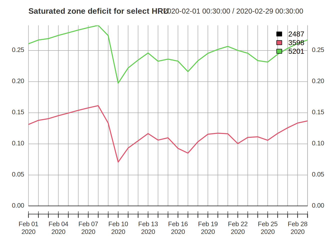

or as a map

## Create a map of the root zone storage at 2020-02-03 02:00:00
s_rz_val <- do.call(rbind, lapply( state_rec[["2020-02-03 00:30:00"]], function(x){ data.frame(id=x$id,s_rz = x$states["s_rz"]) }) )
## create a map of values by substituting s_rz for the id in the hru_id map
hru_id <- rast( file.path(".","dyna","atb_20_model.tif") ) ## open map from from file names stored in the model
s_rz_map<- subst(hru_id, from=s_rz_val$id, to = s_rz_val$s_rz) ## substitute values into the map of HRU id numbers
## and plot
plot(s_rz_map,main="Root zone storage at 2020-02-03 00:30:00")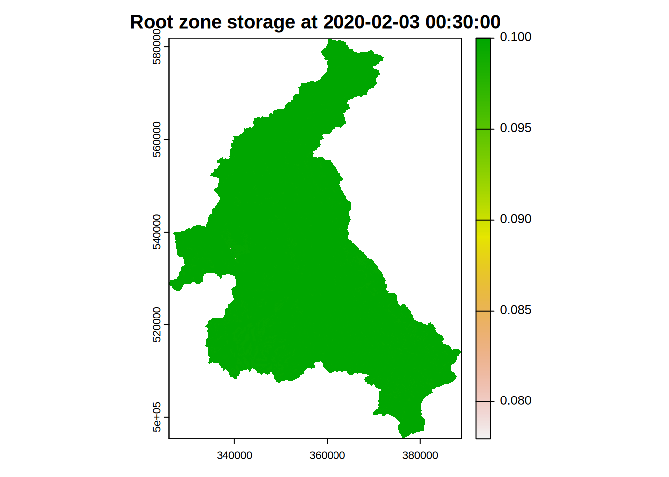

Hot Starting and Saving

Hot starting; that is starting a simulation with the final states of a previous simulation can be achieved by simply not re-initialising the dynatop object before the next call to sim

## initialise and simulate the model
ctch_mdl$initialise()$sim(output_defn)
r1 <- ctch_mdl$get_output() ## get the output from the first run
## run again without initialising
## This will use the final states of the last simulation as the starting states
ctch_mdl$sim(output_defn)
r2 <- ctch_mdl$get_output() ## get the output from the second
plot(r1$Sheepmount)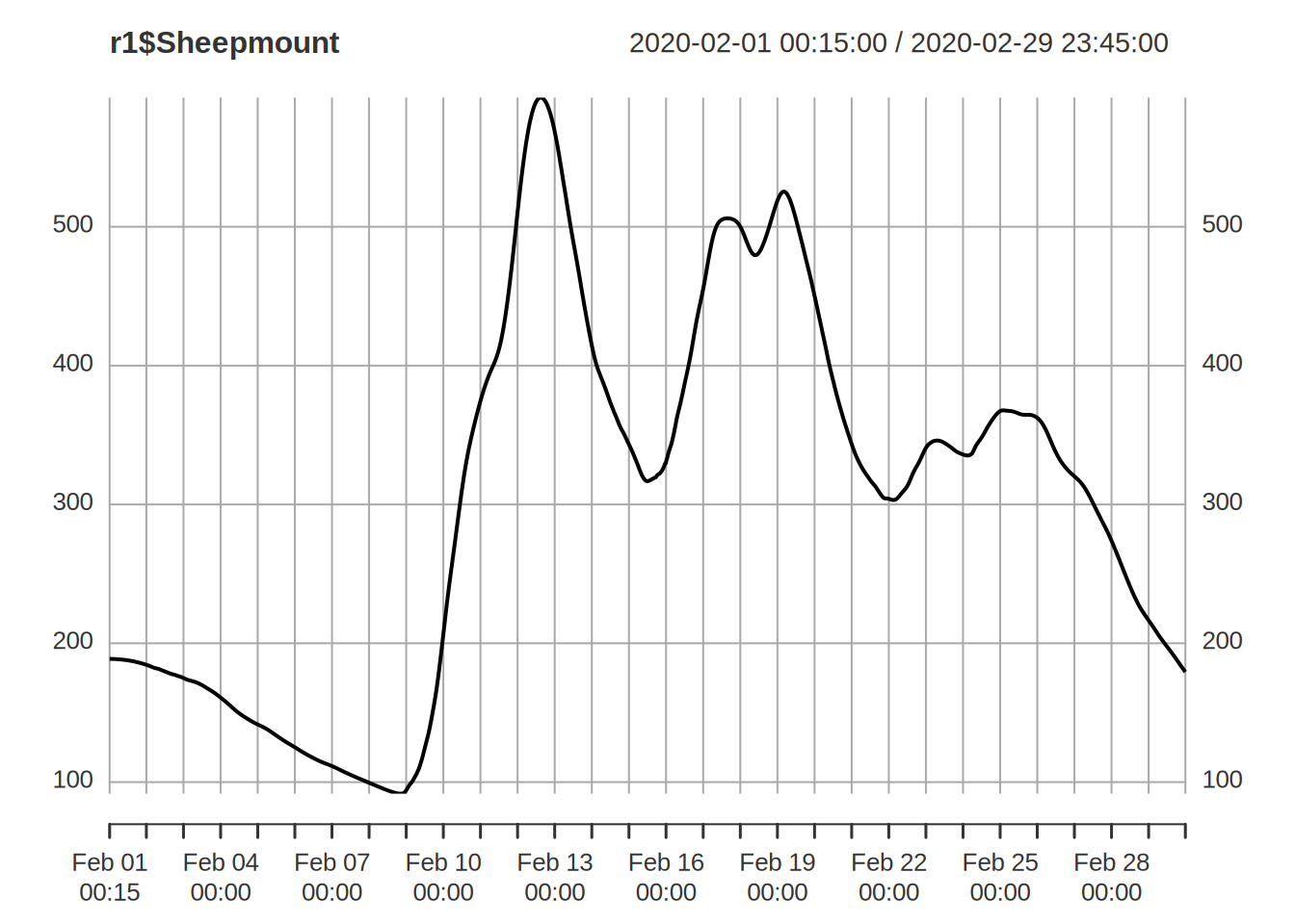

lines(r2$Sheepmount,col="red")## different state values after the second run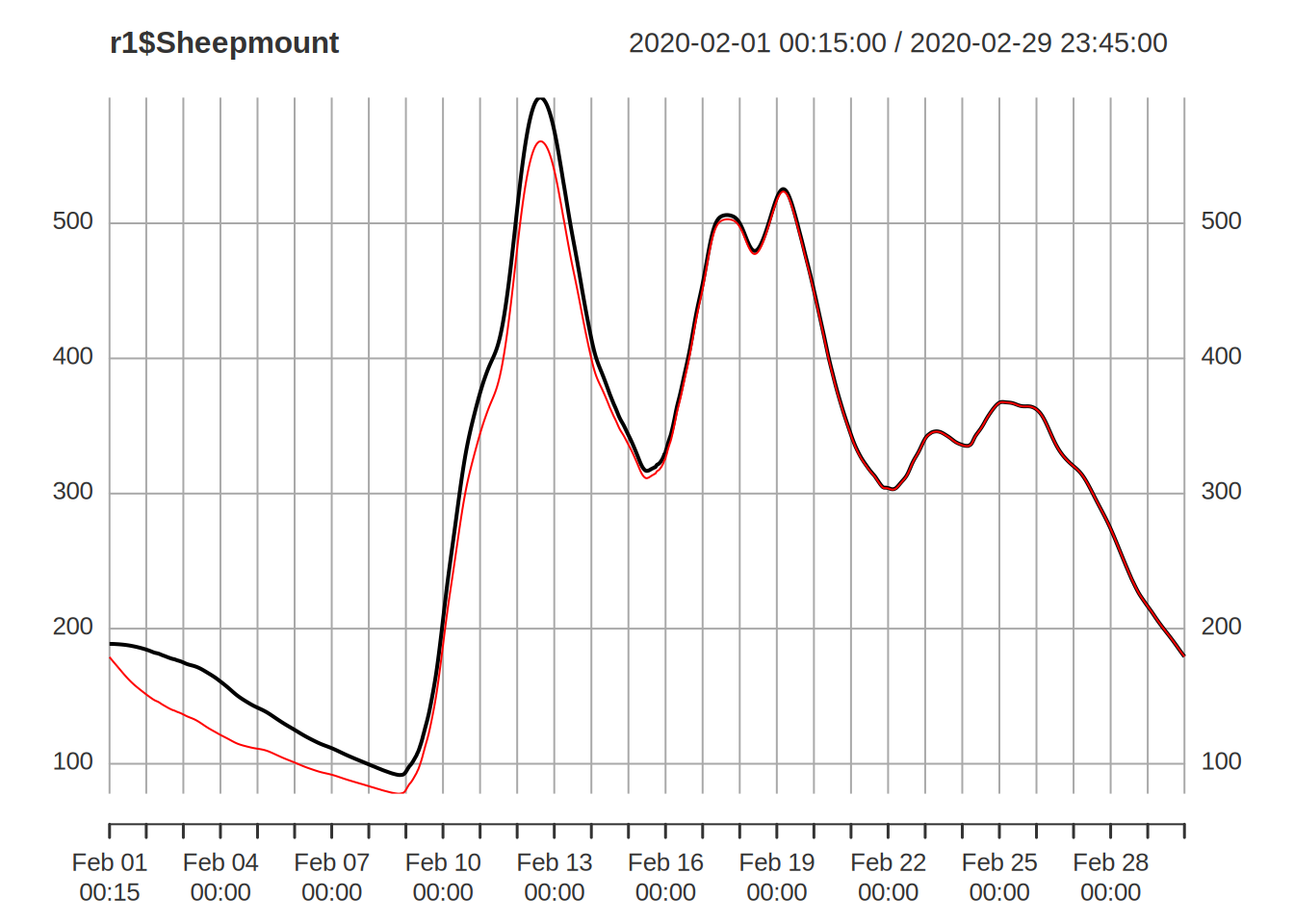

If you want to save the model and current states at the end of a simulation do not save the dynatop object. Instead extract and save he model including the current states and save that.

new_mdl <- ctch_mdl$get_model() ## get the model structure from the dynatop object
new_mdl[[1]] ## as the original model but will final states included
#> $id
#> [1] 0
#> 
#> $states
#>         s_sf         s_rz         s_uz         s_sz 
#> 0.0002078958 0.1000000000 0.0000000000 0.0000000000 
#> 
#> $properties
#>     area    width       Dx gradient 
#>  1.1e+05  2.0e+00  8.4e+02  1.0e-03 
#> 
#> $sf
#> $sf$type
#> cnst 
#>    1 
#> 
#> $sf$parameters
#>  c_sf  d_sf s_raf t_raf 
#>   0.3   0.0   0.0 999.9 
#> 
#> 
#> $rz
#> $rz$type
#> orig 
#>    1 
#> 
#> $rz$parameters
#> s_rzmax 
#>     0.1 
#> 
#> 
#> $uz
#> $uz$type
#> orig 
#>    1 
#> 
#> $uz$parameters
#>   t_d 
#> 28800 
#> 
#> 
#> $sz
#> $sz$type
#> exp 
#>   1 
#> 
#> $sz$parameters
#>   t_0     m 
#> 0.135 0.040 
#> 
#> 
#> $sf_flow_direction
#> $sf_flow_direction$id
#> integer(0)
#> 
#> $sf_flow_direction$fraction
#> numeric(0)
#> 
#> 
#> $sz_flow_direction
#> $sz_flow_direction$id
#> integer(0)
#> 
#> $sz_flow_direction$fraction
#> numeric(0)
#> 
#> 
#> $initialisation
#>       s_rz_0    r_uz_sz_0 
#> 7.500000e-01 8.322539e-08 
#> 
#> $precip
#> $precip$name
#> [1] "precip_76" "precip_75"
#> 
#> $precip$fraction
#> [1] 0.90909091 0.09090909
#> 
#> $precip$idx
#> precip_76 precip_75 
#>        76        75 
#> 
#> 
#> $pet
#> $pet$name
#> [1] "pet"
#> 
#> $pet$fraction
#> [1] 1
#> 
#> $pet$idx
#> pet 
#> 100 
#> 
#> 
#> $class
#> $class$min_dst
#> [1] 1
#> 
#> $class$atb_20_band
#> [1] NA
#> 
#> $class$atb_20
#> [1] NA
#> 
#> $class$band
#> [1] NA
#> 
#> $class$burns
#> [1] NA
#> 
#> $class$name1
#> [1] "Boundary Sike"
#> 
#> $class$name
#> [1] "429B7DBF-B913-4B3B-8001-4A697CFBA416"
#> 
#> $class$startNode
#> [1] "4FA23A32-772E-4B51-873C-0C033989B20A"
#> 
#> $class$endNode
#> [1] "02E2B2F3-5087-48DD-A7E9-41F9B5C7969A"
#> 
#> $class$form
#> [1] "inlandRiver"
#> 
#> $class$flow
#> [1] "in direction"
#> 
#> $class$fictitious
#> [1] "false"
#> 
#> $class$length
#> [1] 840
#> 
#> $class$name2
#> [1] NA
#> 
#> $class$width
#> [1] 2
#> 
#> $class$area
#> [1] 1684.048
#> 
#> $class$slope
#> [1] 0.001
#> 
#> $class$up_area
#> [1] 392924.2
#> 
#> $class$ct_area
#> [1] 392924.2