Dynamic TOPMODEL

This a simplified, opinionated introduction. The original motivation for Dynamic TOPMODEL can be found in Beven & Freer, 2001

Motivation

Dynamic TOPMODEL was originally conceived as “A new version of the rainfall-runoff model TOPMODEL is described in which the assumption of a quasi-steady state saturated zone configuration is replaced by a kinematic wave routing of subsurface flow…” allowing for “…the simulation of dynamically variable up-slope contributing areas.”

Revisiting the idea of TOPMODEL (which has done this mainly for hill slopes, but see Peters et al. 2003) a model is formulated by

• Classifying the catchment up into areas that respond in a hydrologically similar manner
• Determining the connectivity between each of the classes
• Assigning each class to an appropriate Hydrological Representative Unit (HRU), which solves the hydrological processes for a standardised unit

In the following these aspects are outlined with reference to the implementation of Dynamic TOPMODEL in the dynatop and dynatopGIS packages.

Classification and Connectivity

Classification (Part 1)

The location of areas with a hydrological similar response is only every going to be partially captured by spatial data. Past TOPMODEL and Dynamic TOPMODEL applications have used classifications based on a topographic index given by the logarithm of up-slope area divided by the local gradient. Using the up-slope area gives some spatial ordering to the classes, but (as we will see with the Eden data) it is not complete. Consider a small catchment represented by a raster of spatial cells with the following topographic index classes

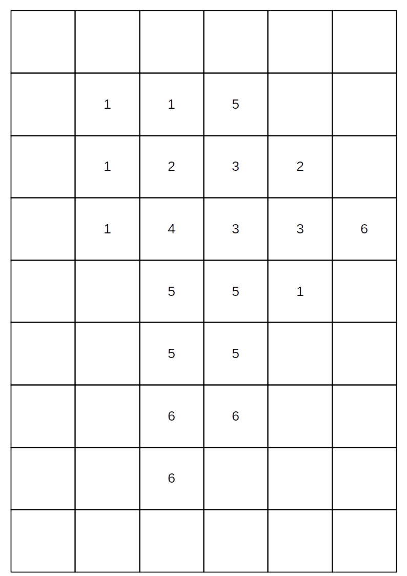
Map of topographic index classes

Since land use could influence the evapotranspiration and infiltration properties a second classification might be desirable. For the small catchment the land use classes are shown below

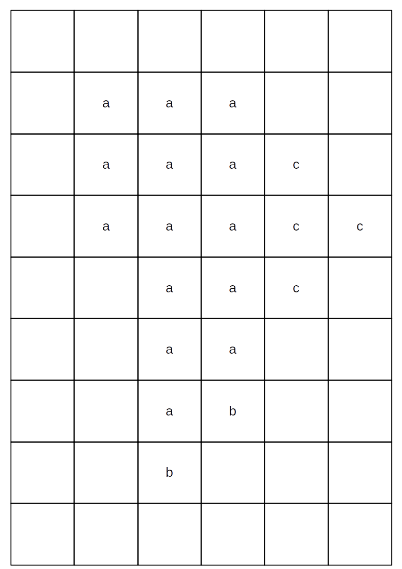
Map of land use classes

Combing these topographic index and land use classes gives one initial class for each unique combination.

Connectivity

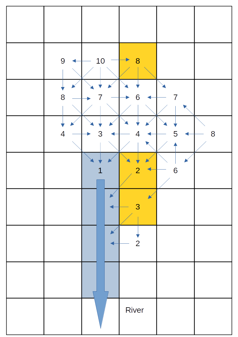
In keeping with earlier spatial analysis TOPMODEL and Dynamic TOPMODEL applications connectivity (flow directions) is assumed to be determined by the surface gradient with any down-slope region receiving flow. This gives a high degree of connectivity between the spatial cells. If a river intercepts a cell it is assumed that both the surface and subsurface flow direction change to follow the river course.The following figure shows the connectivity for the small catchment, with the river cells highlighted in blue.

Map of combined topographic and land use classes along with connectivity

Classification (Part 2)

Each class is represented by a single HRU, the inflows to which are averaged from the inflows to all the spatial cells of that class. Does this make sense for class 5a, which is both in the upper reaches of the catchment but also adjacent to the river?

The dynatop author would argue not. To represent the spatial positioning the catchment can be banded using the connectivity - all cells in a given band receive flows only from those in a higher band. For the small catchment this looks like the following

Map of the band classification

Combing this into the classification gives

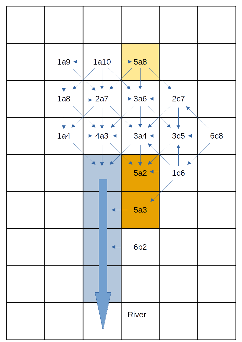
Map of the combined classification

which further separates out the 5a class to the areas close to and further from the river. This demonstrates the banding gives a further level of spatial refinement to the classification while allowing a for simplification in the catchment representation.

Introducing the band into the classification has a further advantage. Solving the HRUs starting with those in the highest band ensures that inflows at the current time step are available for use in the numeric solution. This allow the use of computation techniques that are more robust to the choice of solution time step.

The numeric scheme implemented in the dynatop package makes use of an ordering so that the HRU inflows for the current time step are available. Although other options could be used it is strongly recommended that the default banding scheme is used.

Hydrological Response Units

Each Hydrological Response Unit HRU represents a parameterised version of a different part of the hydrological system. The representation of each HRU is made up of the four zones:

• A Surface Zone representing the movement of water on the surface
• A Root Zone which controls evapotranspiration, handles the precipitation input and flux of water to the unsaturated zone
• A Unsaturated Zone which represented the water between the root zone and the saturated subsurface
• A Saturated Zone representing the saturated subsurface

The following schematic shows the four zones and the fluxes between them

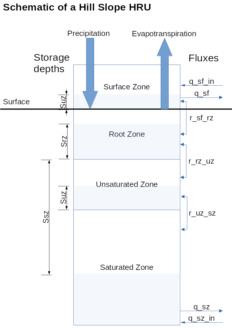
Schematic of the Hill slope HRU

As shown in the schematic fluxes are passed between the HRUs at two levels, the surface and the saturated zones.

To allow for some flexibility in the dynamics of the HRU different representations can be used for each zone. The governing equation and numerical solution of these are given in a vignette of dynatop. A few key points are:

• The lateral flow from the Surface and Saturated Zones is computed using Muskingham approximations.
• Evapotranspiration is proportional to the percentage saturation of the Root Zone
• Flow from the root zone to the Unsaturated Zone can occur only when the Root Zone is full
• The Unsaturated Zone is represented by a tank whose time constant depends upon the deficit of the Saturated Zone
• The lateral flow from the Saturated Zone is controlled by the saturated storage deficit through a transmissivity profile.