Conceptual model
One of the underlying principles of dynamic TOPMODEL is that the landscape can be broken up into hydrologically similar regions, or Hydrological Response Units (HRUs), where all the area within a HRU behaves in a hydrologically similar fashion. Further discussion and the connection of HRUs is outlined elsewhere.
This document outlines the conceptual structure and computational implementation of the HRU. The HRU is a representation of an area of the catchment with, for example, similar topographic, soil and upslope area characteristics.
The HRU is considered to be a area of catchment with outflow occurring across a specified width of it boundary. It is formed of four zones representing the surface water, which passes water between HRUs and drains to the root zone. The root zone characterises the interactions between evapotranspiration and precipitation and when full spills to the unsaturated zone. This drains to the saturated zone which also interacts with other HRUs. The behaviour of the saturated zone is modelled using a kinematic wave approximation. The zones and variables used below are shown in the schematic diagram.
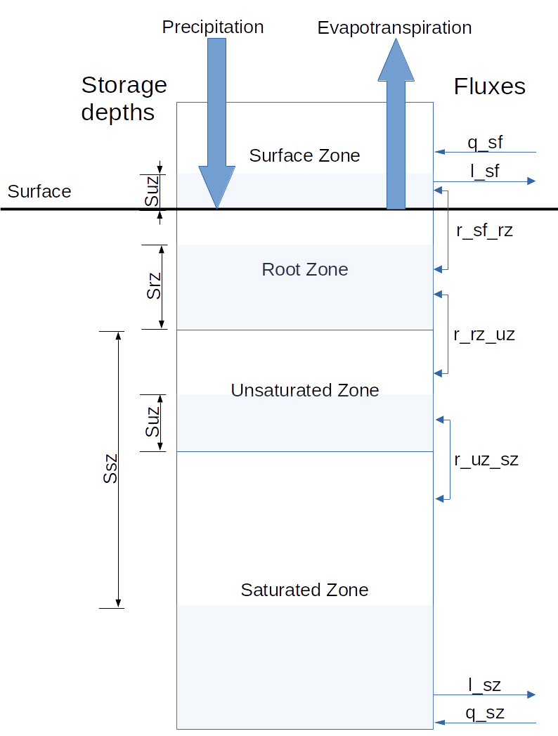
Figure 1: Schematic of the Hill slope HRU
In the following section the governing equations of the HRU are given in a finite volume form. Approximating equations for the solution of the governing equations are then derived with associated implicit and semi-implicit numerical schemes. These are valid for the wide range of surface zone and saturated zone transmissivity profiles presented in the vignette. Appendices provide supporting information.
Notation
Table 1 outlines the notation used for describing an infinitesimal slab across the hillslope HRU.
The following conventions are used:
All properties such as slope angles and time constants are considered uniform along the hillslope.
Precipitation and Potential Evapotranspiration occur at spatially uniform rates.
All vertical fluxes \(r_{\star \rightarrow \star}\) are considered to spatially uniform and to be positive when travelling in the direction of the arrow, but can, in some cases be negative.
All lateral fluxes \(q_{\star}\) and \(q_{\star}\) are considered to be positive flows travelling downslope.
The superscripts \(^+\) and \(^-\) are used to denote variables for the outflow and inflow to the hillslope.
\(\left.y\right\rvert_t\) indicates the value of the variable \(y\) at time \(t\)
| Quantity type | Symbol | Description | unit |
|---|---|---|---|
| Storage | \(s_{sf}\) | Surface excess storage | m\(^3\) |
| \(s_{rz}\) | Root zone storage | m\(^3\) | |
| \(s_{uz}\) | Unsaturated zone storage | m\(^3\) | |
| \(s_{sz}\) | Saturated zone storage deficit | m\(^3\) | |
| Vertical fluxes | \(r_{sf \rightarrow rz}\) | Flow from the surface excess store to the root zone | m\(^3\)/s |
| \(r_{rz \rightarrow uz}\) | Flow from the root zone to the unsaturated zone | m\(^3\)/s | |
| \(r_{uz \rightarrow sz}\) | Flow from unsaturated to saturated zone | m\(^3\)/s | |
| Lateral fluxes | \(q_{sf}\) | Lateral flow in the hillslope surface zone | m\(^3\)/s |
| \(q_{sz}\) | Lateral inflow to the hillslope surface zone | m\(^3\)/s | |
| Vertical fluxes to the HRU | \(p\) | Precipitation rate | m\(^3\)/s |
| \(e_p\) | Potential Evapotranspiration rate | m\(^3\)/s | |
| Other HRU properties | \(A\) | Plan area | m\(^2\) |
| \(w\) | Width of a hill slope cross section | m | |
| \(\Delta x\) | Effective length of the hillslope HRU (x = A/w$) | m | |
| \(\Theta_{sf}\) | Further properties and parameters for the solution of the surface zone | :-: | |
| \(\Theta_{rz}\) | Further properties and parameters for the solution of the root zone | :-: | |
| \(\Theta_{uz}\) | Further properties and parameters for the solution of the saturated zone | :-: | |
| \(\Theta_{sz}\) | Further properties and parameters for the solution of the saturated zone | :-: |
Finite Volume Formulation
In this section a finite volume formulation of the Dynamic TOPMODEL equations is derived for the evolution of the states over the time step \(t\) to \(t + \Delta t\). The lateral flux rates are considered at the start and end of the time step. The vertical flux rates are considered as constant throughout the time step, allowing for a semi-analytical solution of some storage zones.
Surface zone
The storage in the surface zone satisfies the mass balance equation
\[ \frac{ds_{sf}}{dt} = q^{-}_{sf} - r_{sf \rightarrow rz} - q^{+}_{sf} \]
where surface storage is increased by lateral downslope flow from upslope HRUs. Water flows to the root zone at a constant rate \(r_{sf \rightarrow rz}\), unless limited by the available storage at the surface or the ability of the root zone to receive water (for example if the saturation storage deficit is 0 and the root zone storage is full). In cases where lateral flow in the saturated zone produce saturation storage deficits water may be returned from the root zone to the surface giving negative values of \(r_{sf \rightarrow rz}\).
The outflow \(q^{+}_{sf}\) is considered a function of \(q^{-}_{sf}\), \(s_{sf}\), \(r_{sf \rightarrow rz}\) and parameters \(\Theta_{sf}\) denoted by \[ q^{+}_{sf} = \mathcal{F}\left(s_{sf},q^{-}_{sf},r_{sf \rightarrow rz},\Theta_{sf}\right) \] For the purposes the numerical scheme we limit the set to possible functions \(\mathcal{F}\) to those that are non-decreasing with respect to \(s_{sf}\) and take the value \(0\) when \(s_{sf}=0\). More formally \[ \frac{\partial}{\partial s_{sf}} \mathcal{F}\left(s_{sf},q^{-}_{sf},r_{sf \rightarrow rz},\Theta_{sf}\right) \geq 0 \] and \[ \mathcal{F}\left(0,q^{-}_{sf},r_{sf \rightarrow rz},\Theta_{sf}\right) = 0 \]
Root zone
The root zone gains water from precipitation and the surface zone. It loses water through evaporation and to the unsaturated zone. All vertical fluxes are considered to be spatially uniform. The root zone storage satisfies
\[\begin{equation} 0 \leq s_{rz} \leq s_{rzmax} \end{equation}\]
with the governing ODE \[\begin{equation} \frac{ds_{rz}}{dt} = p - \frac{e_p}{s_{rzmax}} s_{rz} + r_{sf\rightarrow rz} - r_{rz \rightarrow uz} \end{equation}\]
Fluxes from the surface and to the unsaturated zone are controlled by the level of root zone storage along with the state of the unsaturated and saturated zones.
For \(s_{rz} \leq s_{rzmax}\) then \(r_{rz \rightarrow uz} \leq 0\). Negative values of \(r_{rz \rightarrow uz}\) may occur only when water is returned from the unsaturated zone due to saturation caused by lateral inflow to the saturated zone.
When \(s_{rz} = s_{rzmax}\) then \[\begin{equation} p - e_p + r_{sf\rightarrow rz} - r_{rz \rightarrow uz} \leq 0 \end{equation}\] In this case \(r_{rz \rightarrow uz}\) may be positive if \[\begin{equation} p - e_p + r_{sf\rightarrow rz} > 0 \end{equation}\] so long as the unsaturated zone can receive the water. If \(r_{rz \rightarrow uz}\) is ‘throttled’ by the rate at which the unsaturated zone can receive water, then \(r_{sf\rightarrow rz}\) is adjusted (potentially becoming negative) to ensure the equality is met.
Unsaturated Zone
The unsaturated zone acts as a non-linear tank subject to the constraint \[\begin{equation} 0 \leq s_{uz} \leq s_{sz} \end{equation}\]
The governing ODE is written as \[\begin{equation} \frac{ds_{uz}}{dt} = r_{rz \rightarrow uz} - \frac{A s_{uz}}{T_d s_{sz}} \end{equation}\]
If water is able to pass freely to the saturated zone, then it flows at the rate \(\frac{A s_{uz}}{T_d s_{sz}}\). In the situation where \(s_{sz}=s_{uz}\) the subsurface below the root zone can be considered saturated, as in there is no further available storage for water, but separated into two parts: an upper part with vertical flow and a lower part with lateral flux.
It is possible that the downward flux is constrained by the ability of the saturated zone to receive water. If this is the case \(r_{uz \rightarrow sz}\) occurs at the maximum possible rate and \(r_{rz \rightarrow uz}\) is limited to ensure that \(s_{uz} \leq s_{sz}\).
Saturated Zone
For a HRU the alteration of the storage in the saturated zone is given in terms of the storage deficit \(s_sz\) as: \[ \frac{ds_{sz}}{dt} = q^{+}_{sz} - r_{sf \rightarrow rz} - q^{-}_{sz} \]
The relationship between the outflow and storage deficit is given \[ q^{+}_{sz} = \mathcal{G}\left(s_{sz},q^{-}_{sz},\Theta_{sz}\right) \] It is assummed that flow increases with storage so \[ - \frac{d}{ds_{sz}} \mathcal{G}\left(s_{sz},q^{-}_{sz},\Theta_{sz}\right) \geq 0 \] while at the maximum storage deficit \(\mathcal{G}\left(D,q^{-}_{sz},\Theta_{sz}\right) = 0\)
Numerical Solution
No analytical solution yet exists for simultaneous integration of the system of ODEs outlined above. In the following an implicit scheme, where fluxes between stores are considered constant over the time step and gradients are evaluated at the final state, is presented.
The basis of the solution is that a gravity driven system will maximise the downward flow of water within each timestep of size \(\Delta t\). Hence on the first downward pass through the stores the maximum downward volumes of the vertical fluxes \(\hat{v}_{* \rightarrow *} = \Delta t \hat{r}_{* \rightarrow *}\) are determined. These then moderated by the solution of the saturated zone, with an upward pass giving the final states.
Downward Pass
Surface excess
The implicit solution of mass balance equation gives
\[ \left. s_{sf} \right\rvert_{t+\Delta t} = \left. s_{sf} \right\rvert_{t} + \Delta t \left( \left. q_{sf}^{-} \right\rvert_{t+\Delta t} - \left. \mathcal{F}\left(s_{sf},q^{-}_{sf},r_{sf \rightarrow rz},\Theta_{sf}\right)\right\rvert_{t+\Delta t} \right) - \left. v_{sf \rightarrow rz} \right\rvert_{t+\Delta t} \]
Since the outflow is 0 when the \(s_sf=0\) the maximum downward flux volume is \[ \left. \hat{v}_{sf \rightarrow rz} \right\rvert_{t+\Delta t} = \left. s_{sf} \right\rvert_{t} + \Delta t \left. q_{sf}^{-} \right\rvert_{t+\Delta t} \]
Root Zone
The implicit formulation for the root zone gives \[\begin{equation} \left. s_{rz} \right.\rvert_{t + \Delta t} = \left( 1 + \frac{e_{p}\Delta t}{s_{rzmax}} \right)^{-1} \left( \left. s_{rz} \right.\rvert_{0} + \Delta t p + v_{sf \rightarrow rz} - v_{rz \rightarrow uz} \right) \end{equation}\]
Since flow to the unsaturated zone occur only to keep \(s_{rz} \leq s_{rzmax}\) then \[\begin{equation} \hat{v}_{rz \rightarrow uz} = \max\left(0, \left. s_{rz} \right.\rvert_{0} + \Delta t \left( p -e_{p}\right) + \hat{v}_{sf \rightarrow rz} - s_{rzmax} \right) \end{equation}\]
Unsaturated Zone
The implicit expression for the unsaturated zone is given in terms of \(\left. s_{uz} \right.\rvert_{t+\Delta t}\) and \(\left. s_{sz} \right.\rvert_{t+\Delta t}\) as
\[\begin{equation} \left. s_{uz} \right.\rvert_{t+\Delta t} = \frac{T_{d}\left. s_{sz} \right.\rvert_{t+\Delta t}}{ T_{d}\left. s_{sz} \right.\rvert_{t+\Delta t} + A \Delta t} \left( \left. s_{uz} \right.\rvert_{t} + v_{rz \rightarrow uz}\right) \end{equation}\]
Since \(\left. s_{uz} \right.\rvert_{t+\Delta t} \leq \left. s_{sz} \right.\rvert_{t+\Delta t}\) this places an additional condition of \[\begin{equation} \left. s_{uz} \right.\rvert_{t} + v_{rz \rightarrow uz} \leq \left. s_{sz} \right.\rvert_{t+\Delta t} + \frac{A \Delta t}{T_d} \end{equation}\]
By mass balance this gives the maximum downward flux volume as \[ \hat{v}_{uz \rightarrow sz} = A\Delta t \min\left( \frac{\left( \left. s_{uz} \right.\rvert_{t} + \hat{v}_{rz \rightarrow uz}\right)} {T_{d}\left. s_{sz} \right.\rvert_{t+\Delta t} + A \Delta t}, \frac{1}{T_{d}} \right) \]
This is a function of \(\left. s_{sz} \right.\rvert_{t+\Delta t}\).
Saturated Zone
Building on the generic solution the implicit scheme for the saturated zone gives
\[ \left. s_{sz} \right\rvert_{t+\Delta t} = \left. s_{sz} \right\rvert_{t} + \Delta t \left( \left. \mathcal{G}\left(s_{sz},q^{-}_{sz},\Theta_{sz}\right)\right\rvert_{t+\Delta t} - \left. q_{sz}^{-} \right\rvert_{t+\Delta t} \right) - \left. v_{uz \rightarrow sz} \right\rvert_{t+\Delta t} \]
Consider the pseudo-function \[ \mathcal{H}\left(z\right) = z - \left. s_{sz}\right.\rvert_{t} + \Delta t \left. q_{sz}^{-} \right\rvert_{t+\Delta t} + A\Delta t \min\left( \frac{\left( \left. s_{uz} \right.\rvert_{t} + \hat{v}_{rz \rightarrow uz}\right)} {T_{d}z + A \Delta t}, \frac{1}{T_{d}} \right) - \\ \Delta t \min\left(q_{sz}^{max},\max\left( 0, 2 \mathcal{G}\left(z,\Theta_{sz}\right) - \left. q_{sz}^{-} \right\rvert_{t+\Delta t} \right)\right) \]
adapted from the approximating equation for the saturated zone storage. In Appendix A it is shown that \(\mathcal{H}\left(z\right)\) is a monotonic increasing function of \(z > 0\) and \(\mathcal{H}\left(D\right) \geq 0\). Hence if \(\mathcal{H}\left(0\right) \lt 0\) unique solution for \(\left. s_{sz}\right.\rvert_{\Delta t}\) can be found. If \(\mathcal{H}\left(0\right) \geq 0\) then the incoming fluxes are enough to produce saturation in the subsurface and \(\left. s_{sz}\right.\rvert_{\Delta t} = 0\).
Maintaining a water (mass) balance and correct limits on the state values depends upon the accuracy of the solution of \(\mathcal{H}\left(z\right)=0\). Since each evaluation of \(\mathcal{H}\left(z\right)\) requires an evaluation of \(\mathcal{G}\) this rapidly become the most expensive part of the code. Use of a numerical scheme which allows mass balance to maintained regardless of the accuracy of the solution of \(\mathcal{H}\left(z\right)=0\) allows scope for compromises based on computational time.
The upward pass presented below is mass conservative so long as \(\mathcal{H}\left(\left. s_{sz}\right.\rvert_{\Delta t}\right)\geq0\). We therefore seek \(z\) which satifies for some tolerance \(\epsilon>0\) \[ \epsilon \geq \mathcal{H}\left(z\right) \geq 0 \] One approach to finding such a value is use a bracketing algorithm. At each iteration the lower and upper limits \(z^{l} < z^{u}\) satisify \(\mathcal{H}\left(z^{l}\right)\leq 0 \leq \mathcal{H}\left(z^{u}\right)\), thus bracket the solution. Iterating (using for example bisection) until \(\mathcal{H}\left(z^{l}\right) \leq \epsilon\) give the approximation \(\left. s_{sz}\right.\rvert_{\Delta t} = z^{u}\).
Upward Pass
Given an estimate of \(\left. s_{sz}\right.\rvert_{\Delta t}\) such that \(\mathcal{H}\left(\left. s_{sz}\right.\rvert_{\Delta t}\right)>0\) compute the vertical flux volumes in the following fashion
\(\left. q_{sz}^{+}\right.\rvert_{t+\Delta t} = \min\left(q_{sz}^{max},\max\left( 0, 2 \mathcal{G}\left(\left. s_{sz}\right.\rvert_{t+\Delta t},\Theta_{sz}\right) - \left. q_{sz}^{-} \right\rvert_{t+\Delta t}\right)\right)\)
\(v_{uz \rightarrow sz} = \left. s_{sz}\right.\rvert_{t} +\Delta t \left(\left. q_{sz}^{+}\right.\rvert_{t+\Delta t} - \left. q_{sz}^{-} \right\rvert_{t+\Delta t}\right) - \left. s_{sz}\right.\rvert_{t+\Delta t}\)
\(\left. s_{uz}\right.\rvert_{t+\Delta t} = \min\left(\left. s_{sz}\right.\rvert_{t+\Delta t},\left. s_{uz}\right.\rvert_{t} + \hat{v}_{rz \rightarrow uz} - v_{uz \rightarrow sz}\right)\)
\(v_{rz \rightarrow uz} = \left. s_{uz}\right.\rvert_{t+\Delta t} -\left. s_{uz}\right.\rvert_{t} + v_{uz \rightarrow sz}\)
\(v_{sf \rightarrow rz} = \min\left(\hat{v}_{sf \rightarrow rz}, s_{rzmax} - \left. \bar{s}_{rz} \right.\rvert_{0} - \Delta t \left( p - e_p \right) + {v}_{rz \rightarrow uz} \right)\)
Solve for \(\left. s_{rz}\right.\rvert_{t+\Delta t}\) using the equation already given.
Compute the volume loss to evapotranspiration as \(\left. v_{e_{p}}\right.\rvert_{t+\Delta t} = \left. s_{rz}\right.\rvert_{t} + v_{sf \rightarrow rz} - v_{rz \rightarrow uz} + \Delta t p - \left. s_{rz}\right.\rvert_{t+\Delta t}\)
This leaves the solution of the surface zone
Surface Zone
Proceeding in a similar fashion to the saturated zone consider the pseudo-function \[ \mathcal{S}\left(w\right) = \left. s_{sf} \right\rvert_{t} + \Delta t \left( \left. q_{sf}^{-} \right\rvert_{t+\Delta t} - \mathcal{F}\left(w,q_{sf}^{-},\frac{\left. v_{sf \rightarrow rz} \right\rvert_{t+\Delta t}}{\Delta t},\Theta_{sf}\right) \right) - \left. v_{sf \rightarrow rz} \right\rvert_{t+\Delta t} - w \] which is monotonically decreasing for \(w \geq 0\) with \(\mathcal{S}\left(0\right)\geq 0\).
A bracketing solution algorithm gives at any iteration \(w^{l} < \left. s_{sf} \right\rvert_{t+\Delta t} < w^{u}\). An initial value of \(w^{u}\) can be computed as \(\left. s_{sf} \right\rvert_{t} + \Delta t\left. q_{sf}^{-} \right\rvert_{t+\Delta t} - \left. v_{sf \rightarrow rz} \right\rvert_{t+\Delta t}\). Iterating until; for some tolerance \(\epsilon>0\); \(w^{u} - w^{l} < \epsilon\) take \(\left. s_{sf}\right.\rvert_{\Delta t} = w^{l}\). In this case \(\mathcal{S}\left(\left. s_{sf}\right.\rvert_{\Delta t}\right) > 0\) hence mass conservation can be maintained by taking \[ \left. q_{sf}^{+} \right\rvert_{t+\Delta t} = \left. q_{sf}^{-} \right\rvert_{t+\Delta t} + \frac{1}{\Delta t}\left( \left. s_{sf} \right\rvert_{t} - \left. v_{sf \rightarrow rz} \right\rvert_{t+\Delta t} - \left. s_{sf}\right.\rvert_{t + \Delta t}\right) \]
Surface Zone Representations
Recall that The storage in the surface zone satisfies the mass balance equation
\[ \frac{ds_{sf}}{dt} = q^{-}_{sf} - r_{sf \rightarrow rz} - q^{+}_{sf} \]
where surface storage is increased by lateral downslope flow from upslope HRUs. Water flows to the root zone at a constant rate \(r_{sf \rightarrow rz}\), unless limited by the available storage at the surface or the ability of the root zone to receive water (for example if the saturation storage deficit is 0 and the root zone storage is full).
The following subsections present various options for the surface zone solution based on the Muskingham approximation method.
The Muskingham method offers a parsimonious for capturing a range of surface dynamics. This section outlines the key equations and shows how they may be used to capture a range of conceptual models.
Muskingham routing can be derived in a number of ways. The surface storage \(s_{sf}\) in a reach or hillslope of length \(\Delta x\) can be expressed in terms of the representative flow \(q_{sf}\) and velocity \(v_{sf}\) as \[ s_{sf} = \frac{q_{sf} \Delta x}{v_{sf}} \] The representative flow is related to the inflow \(q_{sf}^{-}\) and outflow \(q_{sf}^{+}\) using the parameter \(\eta\) through \[ q_{sf} = \eta q_{sf}^{-} + \left(1-\eta\right) q_{sf}^{+} \] which gives \[ s_{sf} = \frac{\Delta x}{v_{sf}} \left(\eta q_{sf}^{-} + \left(1-\eta\right) q_{sf}^{+} \right) \]
Taking vertical inflow \(r\) the mass balance can be written \[ \frac{ds}{dt} = q^{-} + r - q^{+} \] where substitution of \[ q_{sf}^{+} = \max\left(0, \frac{1}{1-\eta}\left(\frac{sv}{\Delta x} - \eta q^{-} \right) \right) \] gives \[ \frac{ds}{dt} = q^{-} + r - \max\left(0, \frac{1}{1-\eta}\left(\frac{sv}{\Delta x} - \eta q^{-} \right) \right) \] where the maximum ensures that outflow is positive.
Approximating Tank Models
Taking \(\eta=0\) gives \[ \frac{ds}{dt} = q^{-} + r - \frac{sv}{\Delta x} \] which is the equation of a tank model with possibly varying time constant \(T = \frac{\Delta x}{v}\)
Approximating Diffusion Wave Routing
Diffuse routing with lateral inflow can be expressed as the parabolic equation (see for example doi:10.1016/j.advwatres.2005.08.008)
\[ \frac{dq}{dt} + c\frac{dq}{dx} - D \frac{d^2 q}{dx^2} = cl - D \frac{dl}{dx} \] where \(l\) is lateral inflow per unit length. Simplify this by considering that the lateral inflow \(r\) uniformly distributed so that \(l=\frac{r}{\Delta x}\) and \(\frac{dl}{dx}=0\) to give
\[ \frac{dq}{dt} + c\frac{dq}{dx} - D \frac{d^2 q}{dx^2} = cl \]
Let us relate this to the Muskingham Solution using the relationship \[ q = \eta q^{-} + \left(1-\eta\right) q^{+} \]
Taking Taylor series expansions for \(q^{-}\) and \(q^{+}\) based on \(q\) gives
\[ q^{+} \approx q + \eta \Delta x \frac{dq}{dx} + \frac{1}{2}\eta^2\Delta x^2 \frac{d^2 q}{dx^2} \] and \[ q^{-} \approx q - \left(1-\eta\right) \Delta x \frac{dq}{dx} + \frac{1}{2}\left(1-\eta\right)^2 \Delta x^2 \frac{d^2 q}{dx^2} \]
Subtracting the expression for \(q^{-}\) from that for \(q^{+}\) gives
\[ q^{-} - q^{+} \approx -\Delta x \frac{dq}{dx} + \frac{1}{2}\left(1-2\eta\right) \Delta x^2 \frac{d^2 q}{dx^2} \]
From the mass balance condition \[ \frac{ds}{dt} \approx \Delta x l -\Delta x \frac{dq}{dx} + \frac{1}{2}\left(1-2\eta\right)\Delta x^2 \frac{d^2 q}{dx^2} \]
Using the expression for storage and relationship between flow and area \[ \frac{dq}{dt} = \frac{dq}{da} \frac{da}{dt} = \frac{c}{\Delta x} \frac{ds}{dt} \]
Then combining this with the approximation produces \[ \frac{dq}{dt} + c\frac{dq}{dx} - \frac{c}{2}\left(1-2\eta\right)\Delta x \frac{d^2 q}{dx^2} \approx c l \]
Comparison to the original diffuse routing equation shows that \[ \eta \approx \frac{1}{2} - \frac{D}{c \Delta x} \]
The value of \(\eta\) is limited to between 0 and \(\frac{1}{2}\). Firstly \(\eta = 1/2\) results from \(D=0\); that is the Kinematic wave equation. Taking \(\eta=0\) produces the maximum dispersion of \(D = \frac{c\Delta x}{2}\), which is given by the linear tank.
Compound Channels
Compound channels are considered as channels with two regimes corresponding to different reltionships between the \(s_{sf}\), \(q_{sf}\) and \(\eta\) depending upon whether \(s_{sf} \leq s_{c}\), for some storage threshold \(s_{1}\). This allows a basic representation of surface storage such as runoff attenuation features, or out of bank channel flow.
In solving this inflow is partitioned to ensure, where possible, \(s_sf > s_{c}\)
Available Formulations
The different formulation available in the model are given in Table 2 with their parameters outlined in Table 3
| Type | Description | Parameters | \(\mathcal{F}\left(s_{sf},q^{-}_{sf},r_{sf \rightarrow rz},\Theta_{sf}\right)\) |
|---|---|---|---|
| cnst | Linear Tank coupled below a constant parameter diffusive wave solutions | \(t_{raf}, s_{raf},c_{sf}, d_{sf}\) | \[\begin{equation}\begin{array}{l} \eta &=& \frac{1}{2} - \frac{d_{sf}}{c_{sf}\Delta x} \\ q^{+}_{sf} &=& \frac{\min\left(s_{sf},s_{raf}\right)}{t_raf} + \max\left(0, \frac{1}{1-\eta}\left( \frac{c_{sf}}{\Delta x}\max\left(0,s_{sf}-s_{raf}\right) - \eta \hat{q}_{sf}^{-} \right) \right) \end{array}\end{equation}\] |
| kin | Linear tank with Kinematic Wave for remaining flow | \(t_{raf}, s_{raf}, n, w_{sf}, g_{sf}\) | \[\begin{equation} \begin{array}{l} q_{sf} &=& \frac{g_{sf}^{1/2}}{n w_{sf}^{2/3}} \left(\frac{\max\left(0,s_{sf}-s_{raf}\right)}{\Delta x}\right)^{5/3} \\ q^{+}_{sf} &=& \frac{\min\left(s_{sf},s_{raf}\right)}{t_raf} + \max\left(0,2\left( q_{sf} - \frac{1}{2} \hat{q}_{sf}^{-} \right) \right) \end{array}\end{equation}\] |
| comp | Two constant parameter diffusive wave solutions | \(v_{sf,1}, d_{sf,1}, s_{1}, v_{sf,2}, d_{sf,2}\) | \[\begin{equation}\begin{array}{l} \eta_{1} &=& \frac{1}{2} - \frac{d_{sf,1}}{v_{sf,1}\Delta x} \\ \eta_{2} &=& \frac{1}{2} - \frac{d_{sf,2}}{v_{sf,2}\Delta x} \\ q^{+}_{sf} &=& \max\left(0, \frac{1}{1-\eta_{1}}\left( \frac{v_{sf,1}}{\Delta x}\max\left(s_{sf},s_{1}\right) - \eta_{1} \hat{q}_{sf,1}^{-} \right) \right) + \max\left(0, \frac{1}{1-\eta_{2}}\left( \frac{v_{sf,2}}{\Delta x}\max\left(0,s_{sf}-s_{1}\right) - \eta_{2} \hat{q}_{sf,2}^{-} \right) \right) \end{array}\end{equation}\] |
| Symbol | Description | unit |
|---|---|---|
| \(t_{raf}\) | Time constant of the runoff attenuation feature | s |
| \(c_{sf}\) | Free flowing surface water velocity | ms\(^{-1}\) |
| \(s_{raf}\) | storage of the runoff attenuation feature | m\(^3\) |
| \(d_{sf}\) | Free flowing surface water diffusion rate | m\(^2\)s\(^{-1}\) |
| \(w_{sf}\) | Width of surface channel | m |
| \(g_{sf}\) | Gradient of surface channel | - |
| \(n\) | Manning \(n\) coefficent for roughness | sm\(^{-1/3}\) |
Saturated Zone representations
The function \(q_{sz\) = (s_{sz},_{sz})$ dscribing
the representative lateral flow is related to the
HRU width through the transmissivity function. Table
4 gives \(\mathcal{G}\left(s_{sz},\Theta_{sz}\right)\) for various the transmissivity profiles present as options within the dynatop
package, the corresponding value to use for the type value
in the saturated zone specification and the additional parameters
required. The additional parameters are defined in Table
5.
Since the subsurface has a kinematic approximation \[ q_{sz}^{+} = \max\left(0, 2\left( q_{sz} - \frac{1}{2} q_{sf}^{-}\right)\right) \]
| Name | \(G\left(\bar{s}_{sz},\Theta_{sz}\right)\) | \(\Theta_{sz}\) |
type value |
Notes | |
|---|---|---|---|---|---|
| Exponential | \(T_{0}w\sin\left(\beta\right)\exp\left(-\frac{\cos\beta}{Am}s_{sz}\right)\) | \(T_0,\beta,m\) | exp | Originally given in Beven & Freer 2001 | |
| Bounded Exponential | \(T_{0}w\sin\left(\beta\right)\left(\exp\left(-\frac{\cos\beta}{Am}s_{sz}\right) - \exp\left(-\frac{\cos\beta}{m}D\right)\right)\) | \(T_0,\beta,m,D\) | bexp | Originally given in Beven & Freer 2001 | |
| Constant Celerity | \(\frac{c_{sz}w}{A}\left(AD-s_{sz}\right)\) | \(c_{sz},D\) | cnst | ||
| Double Exponential | \(T_{0}w\sin\left(\beta\right)\left( \omega\exp\left(-\frac{\cos\beta}{Am}s_{sz}\right) + \left(1-\omega\right)\exp\left(\frac{\cos\beta}{Am_2}s_{sz}\right)\right)\) | \(T_0,\beta,m,m_2,\omega\) | dexp |
| Symbol | Description | unit |
|---|---|---|
| \(T_0\) | Transmissivity at saturation | m\(^2\)/s |
| \(m\),\(m_2\) | Exponential transmissivity constants | m\(^{-1}\) |
| \(\beta\) | Angle of hill slope | rad |
| \(c_{sz}\) | Saturated zone celerity | m/s |
| \(D\) | Storage deficit at which zero lateral flow occurs | m |
| \(\omega\) | weighting parameter | - |
Appendix A - Monotonicity of \(\mathcal{H}\left(z\right)\)
By definition \(\left. s_{uz} \right.\rvert_{t}\), \(\Delta t\), A, \(T_d\), \(\hat{v}_{rz \rightarrow uz}\) and \(z\) are all greater or equal to 0. To show that the gradient of
\[ \mathcal{H}\left(z\right) = z - \left. s_{sz}\right.\rvert_{t} + \Delta t \left. q_{sz}^{-} \right\rvert_{t+\Delta t} + A\Delta t \min\left( \frac{\left( \left. s_{uz} \right.\rvert_{t} + \hat{v}_{rz \rightarrow uz}\right)} {T_{d}z + A \Delta t}, \frac{1}{T_{d}} \right) - \\ \Delta t \min\left(q_{sz}^{max},\max\left( 0, 2 \mathcal{G}\left(z,\Theta_{sz}\right) - \left. q_{sz}^{-} \right\rvert_{t+\Delta t} \right)\right) \]
is strictly positive consider first the gradient of the last term which takes the value
\[ \frac{d}{dz} \min\left(q_{sz}^{max},\max\left( 0, 2 \mathcal{G}\left(z,\Theta_{sz}\right) - \left. q_{sz}^{-} \right\rvert_{t+\Delta t} \right)\right) = \left\{ \begin{array}{cl} 0 & 2 \mathcal{G}\left(z,\Theta_{sz}\right) < \left. q_{sz}^{-} \right\rvert_{t+\Delta t}\\ 0 & 2 \mathcal{G}\left(z,\Theta_{sz}\right) - \left. q_{sz}^{-} \right\rvert_{t+\Delta t}> q_{sz}^{max} \\ 2 \frac{d}{dz} \mathcal{G}\left(z,\Theta_{sz}\right) & \mathrm{otherwise} \end{array} \right. \]
By definition \(-\frac{d}{dz} \mathcal{G}\left(z,\Theta_{sz}\right) \geq 0\) hence
\[ \frac{d}{dz} \mathcal{H}\left(z\right) \geq 1 + A\Delta t \frac{d}{dz} \min\left( \frac{\left( \left. s_{uz} \right.\rvert_{t} + \hat{v}_{rz \rightarrow uz}\right)} {T_{d}z + A \Delta t}, \frac{1}{T_{d}} \right) \]
Separating the range of \(z\) into two sections gives
\[ \frac{d}{dz} \mathcal{H}\left(z\right) \geq \left\{ \begin{array}{cl} 1 & \frac{\left( \left. s_{uz} \right.\rvert_{t} + \hat{v}_{rz \rightarrow uz}\right)} {T_{d}z + A \Delta t} \geq \frac{1}{T_{d}} \\ 1 - T_{d} A\Delta t \frac{\left. s_{uz} \right.\rvert_{t} + \hat{v}_{rz \rightarrow uz}} {\left(T_{d}z + A \Delta t\right)^2} & frac{\left( \left. s_{uz} \right.\rvert_{t} + \hat{v}_{rz \rightarrow uz}\right)}{T_{d}z + A \Delta t} \leq \frac{1}{T_{d}} \end{array} \right. \]
Further using the range of \(z\) valid for the second case
\[ \frac{d}{dz} \mathcal{H}\left(z\right) \geq \left\{ \begin{array}{cl} 1 & \frac{\left( \left. s_{uz} \right.\rvert_{t} + \hat{v}_{rz \rightarrow uz}\right)} {T_{d}z + A \Delta t} \geq \frac{1}{T_{d}} \\ 1 - \frac{A\Delta t}{T_{d}z + A \Delta t} & \frac{\left( \left. s_{uz} \right.\rvert_{t} + \hat{v}_{rz \rightarrow uz}\right)}{T_{d}z + A \Delta t} \leq \frac{1}{T_{d}} \end{array} \right. \]
From this it can be seen that \(\frac{d}{dz} \mathcal{H}\left(z\right) \geq 0\) with equality possible when \(z=0\).