Using Dynamic TOPMODEL • dynatop

The purpose of this vignette is to provide an outline of the steps needed to perform a Dynamic TOPMODEL simulation and introduce the formats of the data input and returned.

The data used in this example comes from Swindale and is contained within the package and can be loaded with

library(dynatop)
data("Swindale")

which returns a variable Swindale with the following components:

names(Swindale)
#> [1] "model" "obs"

For better comparison with a likely analysis we separate these into a model and observed data variables

swindale_model <- Swindale$model
swindale_obs <- Swindale$obs

The model structure

A dynamic TOPMODEL is described in a list object. The list has the following elements

names(swindale_model)
#> [1] "hru"         "output_flux" "map"

which are described in associated vignette. The dynatopGIS package can be used for constructing models.

Setting map locations

While not required for simulations if the location of a file containing the a raster map of the locations of the HRUs is provided the states can be visualised within dynatop.

The locations of the files are set in the map element of the model. For this example the maps are located within the extdata directory of the package and can be set using commands

swindale_model$map <- system.file("extdata","Swindale.tif",package="dynatop",mustWork=TRUE)

Preparing input data

The input to the model is expected to take the form of an xts object with constant time step whose column names are found in the ‘precip’ and ‘pet’ variables of the HRUs descriptions in the model. Helpful functions for creating and manipulating xts objects can be found here, see also the resample_xts function in this package.

The discharge, precipitation and potential evapotranspiration (PET) inputs for Swindale are contained with swindale_obs on a 15 minute time step.

head(swindale_obs)
#> Warning: object timezone ('GMT') is different from system timezone ('UTC')
#>   NOTE: set 'options(xts_check_TZ = FALSE)' to disable this warning
#>     This note is displayed once per session
#>                     flow precip          pet
#> 2009-11-18 16:00:00 2.78  4e-04 8.878467e-06
#> 2009-11-18 16:15:00 2.80  2e-04 4.762229e-06
#> 2009-11-18 16:30:00 2.85  4e-04 8.585708e-07
#> 2009-11-18 16:45:00 2.94  2e-04 0.000000e+00
#> 2009-11-18 17:00:00 3.02  2e-04 0.000000e+00
#> 2009-11-18 17:15:00 3.15  2e-04 0.000000e+00

Note the discharge is in m\(^{3}\)/s while the precipitation and PET are in m accumulated over the time step.

To use the data with the model we need to set the names of the time series inputs within the model. In this case this is already done as can be seen by inspecting the precip and pet values for the individual HRU’s

head(swindale_model$hru[[1]]$precip)
#> $name
#> [1] "precip"
#> 
#> $fraction
#> [1] 1
head(swindale_model$hru[[1]]$pet)
#> $name
#> [1] "pet"
#> 
#> $fraction
#> [1] 1

Altering parameters

The parameter values are stored within the HRU descriptions. Which parameters are present depends upon the options selected for the transmissivity and channel solution. Details can be found in the HRU Vignettes.

Altering parameter values requires changing their values in the HRU definitions. For this catchment all HRU have the same parameter values. For this simulation we change the parameter vectors to be more representative of the catchment

hru <- swindale_model$hru
for(ii in 1:length(hru)){
    if(is.na(hru[[ii]]$class$endNode)){
        ## then HRU is not a channel
        ## saturated zone parameters
        hru[[ii]]$sz$parameters["m"] <- 0.0063
        hru[[ii]]$sz$parameters["t_0"] <- exp(7.46)
        ## unsaturated zone parameters
        hru[[ii]]$uz$parameters["t_d"] <- 8*60*60
        ## root zone parameters
        hru[[ii]]$rz$parameters["s_rzmax"] <- 0.1
        ## surface parameters
        hru[[ii]]$sf$parameters["c_sf"] <- 0.4
    }else{
        ## then HRU is a channel - set so no subsurface response
        ## saturated zone parameters
        hru[[ii]]$sz$parameters["t_0"] <- 0.001
        ## root zone parameters
        hru[[ii]]$rz$parameters["s_rzmax"] <- 0.001
        ## surface parameters
        hru[[ii]]$sf$parameters["c_sf"] <- 0.8
    }
    ## initialisation parameters
    hru[[ii]]$initialisation["s_rz_0"] <- 0.98
    hru[[ii]]$initialisation["r_uz_sz_0"] <- 1.755582e-07 ## initial outflow divided by catchment area
}

Creating the dynatop Object

Simulations are performed by embedding the model and the observed data into a dynatop object. First the object is created using the model in list form

ctch_mdl <- dynatop$new(hru,map=swindale_model$map)

This step performs some basic checks on the model for consistency. The data can then be added

ctch_mdl$add_data(swindale_obs)

Running dynamic TOPMODEL

The model can be run with the sim method. The methods check that suitable input data is available, but not how it was generated.

The initial states of the simulations can be specified in the model object. If, as in the case of this example, the states are not specified then any attempt to perform a simulation will fail.

ctch_mdl$sim(swindale_model$output_flux)
#> Warning in private$digest_output_defn(output_defn): Output definition does not
#> have scale - adding a vector of 1's
#> Error in ctch_mdl$sim(swindale_model$output_flux): Model states have non-finite values

Rather then editing each HRU to provide states they can be initialised using the initialise method which requires an initial recharge rate to be set for each HRU. In the following we initialise the states and plot the initial saturated zone storage deficit, using the chaining of commands.

ctch_mdl$initialise()$plot_state("s_sz")

The simulation can now be performed and the flow at the gauge extracted with

sim1 <- ctch_mdl$sim(swindale_model$output_flux)$get_output()
#> Warning in private$digest_output_defn(output_defn): Output definition does not
#> have scale - adding a vector of 1's

Note that the states of the system are now those at the end of the simulation for example:

ctch_mdl$plot_state("s_sz")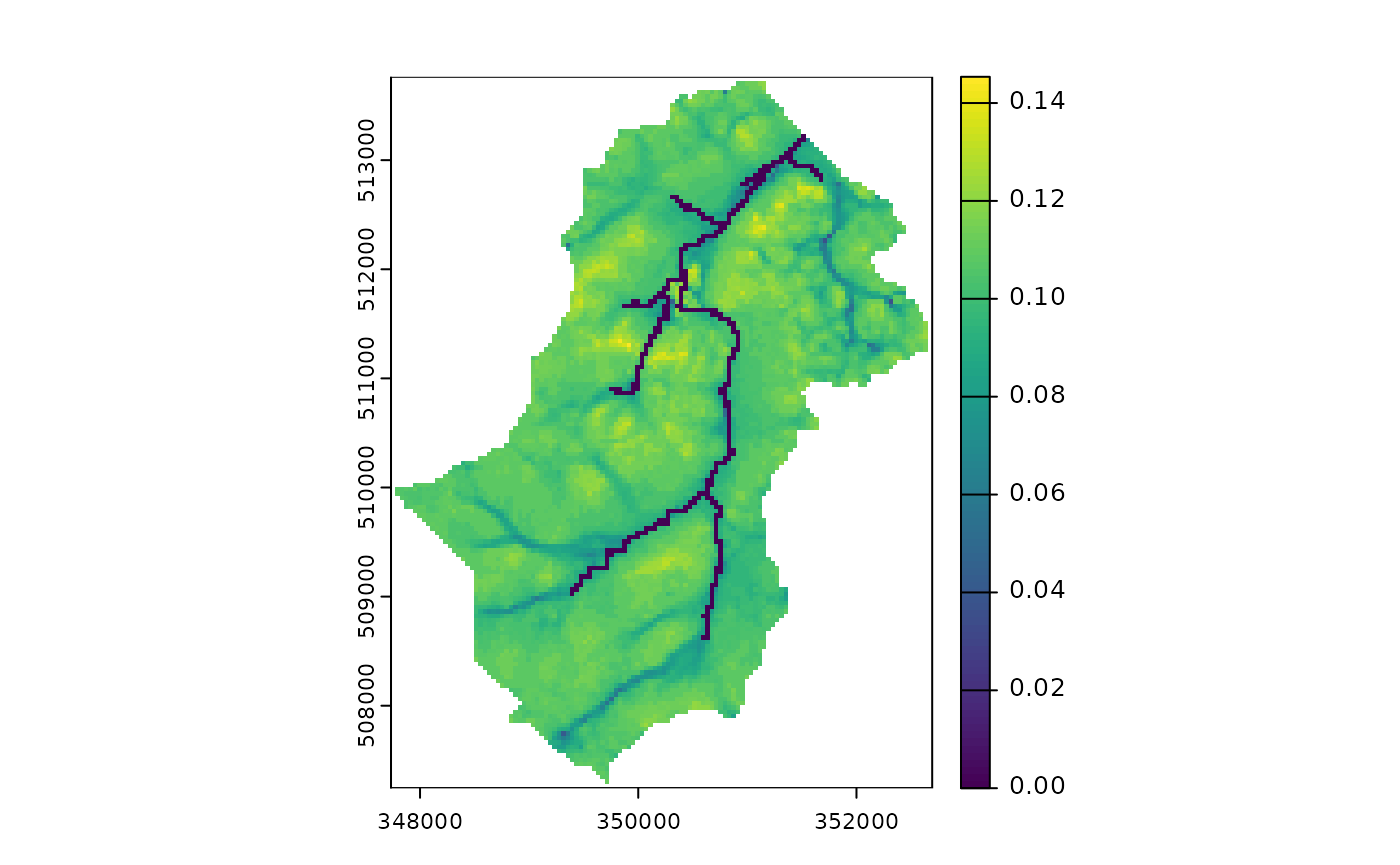

Rerunning the simulation with the new initial states will of course produce different results. Output for the above examples can be plotted against observed discharge for comparison as follows:

sim2 <- ctch_mdl$sim(swindale_model$output_flux)$get_output()
#> Warning in private$digest_output_defn(output_defn): Output definition does not
#> have scale - adding a vector of 1's
out <- merge( merge(swindale_obs,sim1),sim2)
names(out) <- c(names(swindale_obs),'sim_1','sim_2')
plot(out[,c('flow','sim_1','sim_2')], main="Discharge",ylab="m3/s",legend.loc="topright")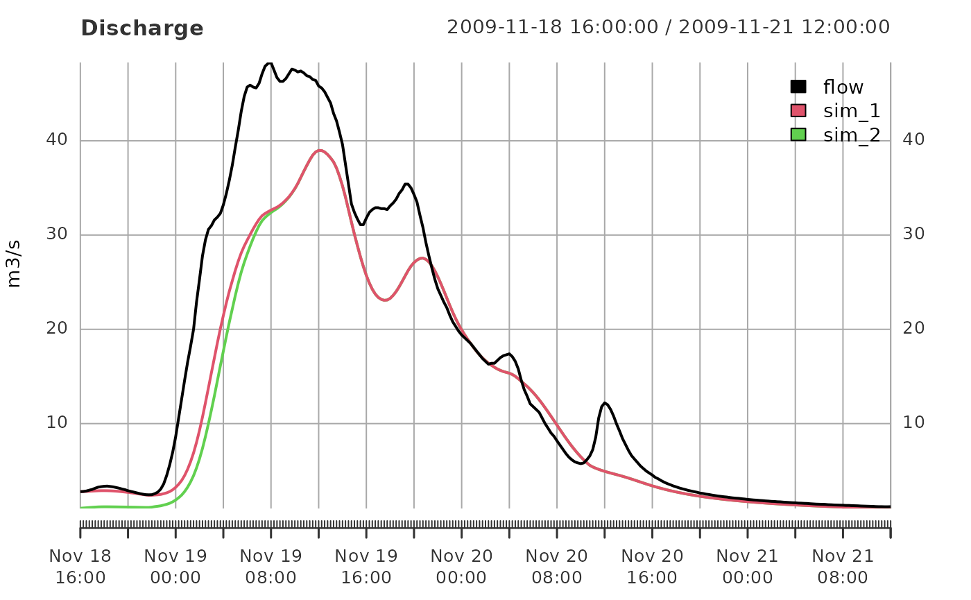

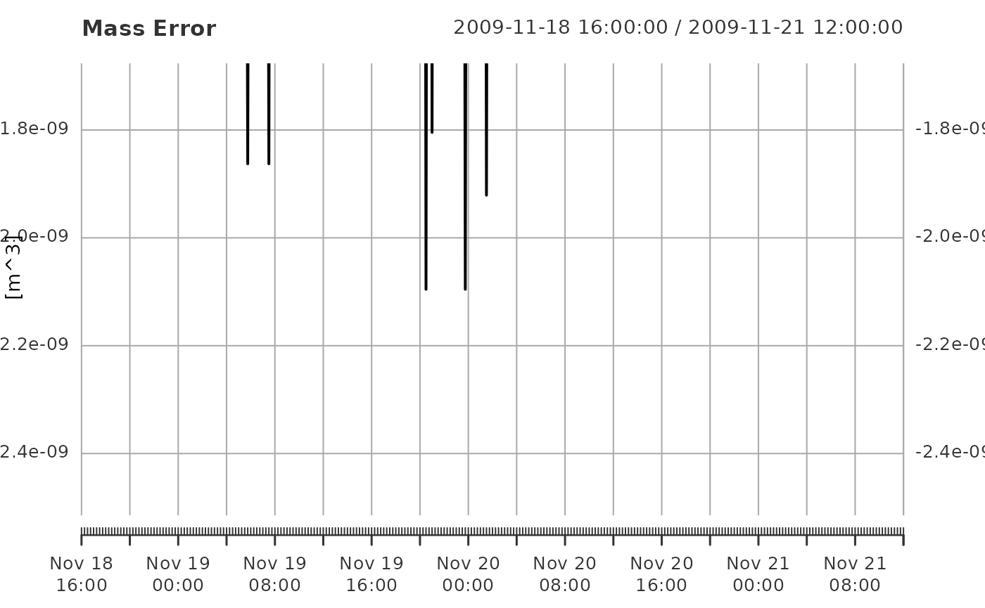
Mass balance

It is possible to output the mass balance check for each time step of the simulation using the get_mass_errors method. The returned xts object gives the volumes in the states at the start and end of the time step along with the other fluxes as volumes. This can easily be used to plot the errors as shown below.

mb <- ctch_mdl$get_mass_errors()
plot( mb[,6] , main="Mass Error", ylab="[m^3]")