Initial GIS processing

Aim

To explore and pre-process the GIS data for the Eden catchment.

Required R Packages

R has multiple packages for the processing and analysis spatial data. A good overview is given in the Spatial Task View on CRAN. For this part of the training course we use a set of mature package terra which is a dependency of dynatopGIS. Similar results could be generated with other packages.

Attached the terra package to the R environment so that its functions are available.

library(terra)
#> terra 1.7.71
library(dynatopGIS)

and remember to move to the eden_data directory e.g.

setwd("../eden_data")

Data Required by `dynatopGIS`

To build a Dynamic TOPMODEL the dynatopGIS package requires the following

A raster map of the catchment, possibly delineating sub-catchments
A raster DEM covering the catchment
A vector polygon representation of the river network

Optionally the user can also provide

A raster map delineating spatial rainfall patterns
A raster map delineating spatial PET patterns
Raster maps containing further data to help classify the HRUs

All raster data must in the same resolution and projection as the catchment map. The vector river data must have the same projection.

dynatopGIS only works with projected raster data with square cells and assumes all raster values are numeric! The raster map of the catchment should have only NA values in the edge row and columns.

Loading Data

There are four types of spatial data in the example; raster, polygons, lines and points; in three different formats; Geotiff, shapefile and csv.

To start use functions in the raster package to load both the raster data and that contained in the shapefiles:

dem <- rast(file.path(".","unprocessed","Eden_DEM.tif")) # load the dem as a raster layer
eden <- vect(file.path(".","unprocessed","Eden_Catchment.shp")) # load the outline of the sub-catchments from the shapefile
channel <- vect(file.path(".","unprocessed","Eden_River_Network.shp")) # load the river network from the shapefile
urban <- vect(file.path(".","unprocessed","Eden_Urban.shp")) # load the urban area map from the shapefile

Typing the variable name at the R prompt will display a summary of the data loaded, for example

dem
#> class       : SpatRaster 
#> dimensions  : 863, 629, 1  (nrow, ncol, nlyr)
#> resolution  : 100, 100  (x, y)
#> extent      : 326000, 388900, 495450, 581750  (xmin, xmax, ymin, ymax)
#> coord. ref. : OSGB36 / British National Grid (EPSG:27700) 
#> source      : Eden_DEM.tif 
#> name        : Eden_DEM 
#> min value   :   -2.700 
#> max value   :  923.425

Compare the dem, eden, channel and urban variable to check that:

there is a common projection
the cells of DEM are square

Reading the gauge locations from the csv file is a two stage process

 # read in the csv file to a date.frame
csvGauges <- read.csv(file.path(".","unprocessed","Eden_Gauge_Sites.csv"))
# convert the data frame to a SpatVect object - take projection from the DEM
gauges <- vect(csvGauges,geom=c("x","y"),crs=crs(dem))

Next plot the data using the default methods in the raster package

plot(dem) # underlying coloured image with scale
plot(urban,add=TRUE,col="grey") # grey polygons
plot(channel,add=TRUE,col="blue") # channels as blue lines
plot(eden,add=TRUE) # outlines of sub-catchments in black
plot(gauges,add=TRUE,col="red") # gauges as red dot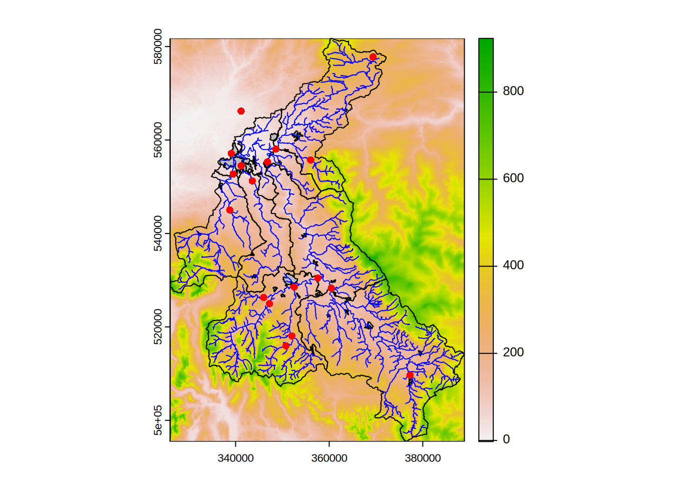

Rasterising Layers

The basis of the landscape discretisation is the raster catchment map. In this example, as in many situation the catchment outlines are vectors shapes. These are rasterised using the grid provided by the raster DEM. In the catchment map each sub-catchment requires a unique numeric value which is provided by the id field.

## show data frame with id values
head(eden)
#>      id                     label
#> 1 76007        Eden at Sheepmount
#> 2 76003          Eamont at Udford
#> 3 76005    Eden at Temple Sowerby
#> 4 76017       Eden at Great Corby
#> 5 76008     Irthing at Greenholme
#> 6 76010 Petteril at Harraby Green
## rasterise
eden_raster <- rasterize(eden, dem, field="id")
## plot the resulting raster
plot(eden_raster)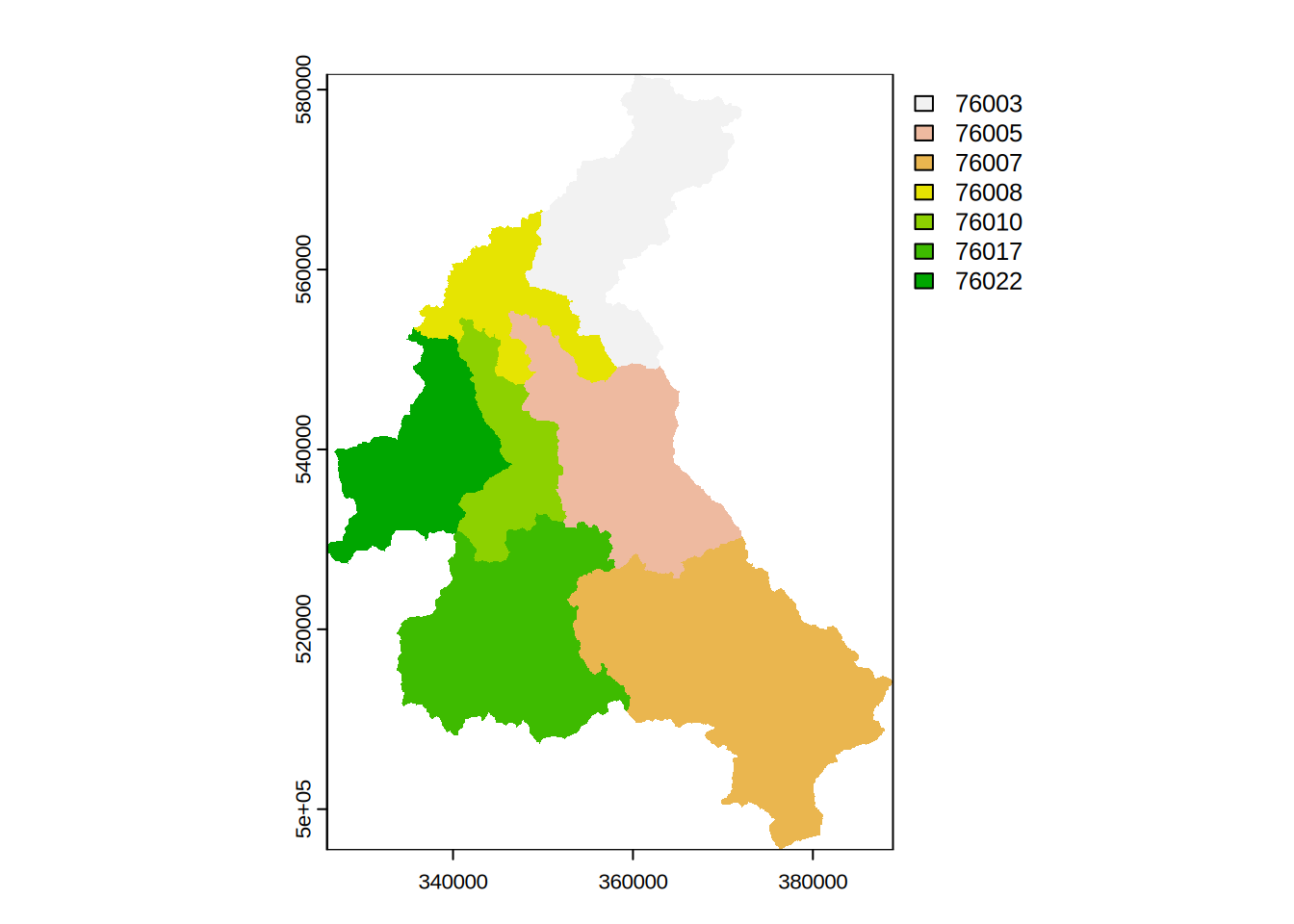

To ensure the edges are NA values the raster is extended, along with that of the DEM

eden_raster <- extend(eden_raster,1)
dem <- extend(dem,1)

Since the urban areas may be used in the classification they are also rasterised. Suitable numeric values are taken from the unique identifiers in the data.

In the case of the urban data there are two possible identifiers objectid and bua_id:

## show data frame with id values
head(urban)
#>   objectid   bua11cd            bua11nm bua_id has_sd sd_count urban_bua
#> 1       39 E34000039        Penrith BUA    747      N        0       Yes
#> 2       47 E34000047  Brough (Eden) BUA   1465      N        0        No
#> 3      297 E34000297       Gilsland BUA   4584      N        0        No
#> 4      869 E34000869        Lazonby BUA   1016      N        0        No
#> 5      899 E34000899 Kirkby Stephen BUA   1359      N        0        No
#> 6      986 E34000986        Dalston BUA    919      N        0        No
#>   st_areasha st_lengths
#> 1  4647359.1  19399.690
#> 2   324993.0   5799.919
#> 3   214996.1   3499.903
#> 4   412499.4   5600.042
#> 5   692492.4   9500.029
#> 6   582500.1   7699.932
## rasterise using objectid as the raster value
urban_raster <- rasterize(urban, eden_raster, field="objectid")
## plot the resulting raster
plot(urban_raster)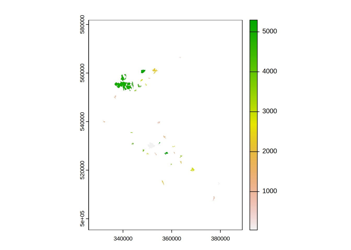

The raster fields created (eden_raster, urban_raster and extended dem) exist only in memory (or temporary files). Since they will be needed later we will save them:

writeRaster(eden_raster,file.path(".","processed","eden.tif"),overwrite=TRUE)
writeRaster(urban_raster,file.path(".","processed","urban.tif"),overwrite=TRUE)
writeRaster(dem,file.path(".","processed","dem.tif"),overwrite=TRUE)

Channel Network

The channel network in the dynamic TOPMODEL generated by dynatopGIS is a series of connected HRUs each representing a single reach length. In the processing done by dynatopGIS each reach is represented by a single spatial polygon. The data for each reach must include the following fields:

name - The unique identifier/name of the reach
length - Length of the reach [m]
startNode - An identifier for the head of the reach
endNode - An identifier for the foot of the reach
width - Channel width [m]
slope - Channel slope [m/m]

The startNode and endNode values are used to define the channel connectivity, while the physical properties are used in the dynatop numerical solutions.

Looking at the channel data

channel
#>  class       : SpatVector 
#>  geometry    : lines 
#>  dimensions  : 1697, 9  (geometries, attributes)
#>  extent      : 327613.4, 388606.5, 496531.8, 581285.4  (xmin, xmax, ymin, ymax)
#>  source      : Eden_River_Network.shp
#>  coord. ref. : OSGB36 / British National Grid (EPSG:27700) 
#>  names       :          name1      identifier       startNode         endNode
#>  type        :          <chr>           <chr>           <chr>           <chr>
#>  values      :             NA 71496043-333C-~ 785AA707-7ACC-~ FD4A9B62-950E-~
#>                Rowantree Gill C1E710A3-ED27-~ FD4A9B62-950E-~ 323B8FBC-8D31-~
#>                     Lady Sike 0B92A0E8-4B7B-~ 76150301-B4E4-~ 41DAD94A-AF47-~
#>         form         flow fictitious length name2
#>        <chr>        <chr>      <chr>  <int> <chr>
#>  inlandRiver in direction      false     31    NA
#>  inlandRiver in direction      false    986    NA
#>  inlandRiver in direction      false    321    NA

we see that it already contains

an identifier for the foot of the reach called endNode
an identifier for the head of the reach called startNode
the reach length
a unique identifier called identifier

but is composed to spatial lines rather then polygons.

The dynatopGIS package provides a function for conveniently converting line objects to the correct format.

conv_channel <- convert_channel(
    channel,
    property_names = c(name = "identifier", length = "length", startNode = "startNode",
                       endNode= "endNode"),
    default_width = 2,
    default_slope = 0.001
)
#> Warning in convert_channel(channel, property_names = c(name = "identifier", :
#> Modifying to spatial polygons using default width
#> Warning in convert_channel(channel, property_names = c(name = "identifier", :
#> Adding default slope

The two warning messages reveal that, since they are not specified, default width and slope values are added. The width property is used to buffer the channel resulting in spatial polygons.

conv_channel
#>  class       : SpatVector 
#>  geometry    : polygons 
#>  dimensions  : 1697, 12  (geometries, attributes)
#>  extent      : 327612.4, 388607.5, 496530.8, 581286.4  (xmin, xmax, ymin, ymax)
#>  coord. ref. : OSGB36 / British National Grid (EPSG:27700) 
#>  names       :          name1            name       startNode         endNode
#>  type        :          <chr>           <chr>           <chr>           <chr>
#>  values      :             NA 71496043-333C-~ 785AA707-7ACC-~ FD4A9B62-950E-~
#>                Rowantree Gill C1E710A3-ED27-~ FD4A9B62-950E-~ 323B8FBC-8D31-~
#>                     Lady Sike 0B92A0E8-4B7B-~ 76150301-B4E4-~ 41DAD94A-AF47-~
#>         form         flow fictitious length name2 width  area slope
#>        <chr>        <chr>      <chr>  <num> <chr> <num> <num> <num>
#>  inlandRiver in direction      false     31    NA     2 64.69 0.001
#>  inlandRiver in direction      false    986    NA     2  1975 0.001
#>  inlandRiver in direction      false    321    NA     2 645.2 0.001

The converted channel data is saved for later use

writeVector(conv_channel,file.path(".","processed","channel.shp"),overwrite=TRUE)

The use of polygons to represent channel sections allows the shape of water features such as lakes to be captured

Locating Gauges on the Channel Network

Before locating the gauges on the network note that in the map of the loaded data there is a single gauge outside to the catchment area. As simple example of manipulating spatial data in R is to remove this by cropping the gauges to the catchment area. This is done by

gauges <- crop(gauges,eden)

To determine the location of the gauges on the river network we identify for each gauge the closest reach. The identifier of this reach, along with the distance to the gauge data is then added to the gauge data.

dst <- distance(gauges,conv_channel) ## distance between gauges(row) and channels(column)
idx <- apply(dst,1,which.min) ## index of closest channel for each gauge

gauges$chn_identifier <- conv_channel$name[ apply(dst,1,which.min) ]
gauges$chn_distance <- apply(dst,1,min) ## distance to the channel

To check the results by plotting:

selected <- conv_channel[conv_channel$name %in% gauges$chn_identifier,]
plot(eden) # outlines of sub-catchments in black
plot(conv_channel,add=TRUE,col="blue",border="blue") # channel network in blue
plot(selected,add=TRUE,col="orange",border="orange") # selected reachs in orange
plot(gauges,add=TRUE,col="red",pch=21) # gauges as red filled circles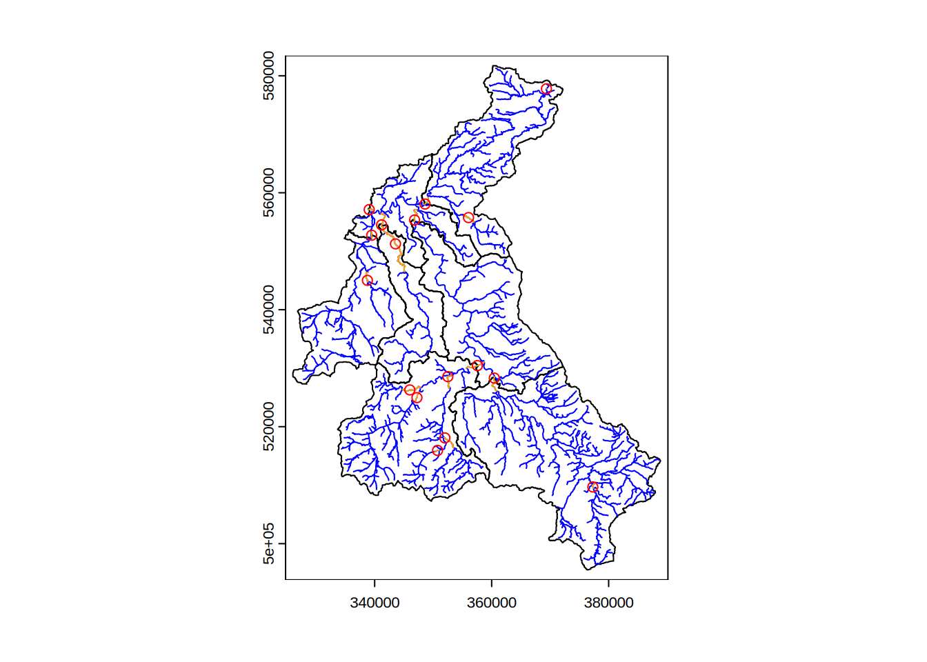

The cropped list of gauges with channel identifier can be saved to a shapefile:

writeVector(gauges,file.path(".","processed","gauges.shp"),overwrite=TRUE)

The quality of results of any method used for any automatic method of locating the gauges depends upon the accuracy of the GIS data.

In the numeric solution used in dyantop it is assumed that a gauge is at the foot of a reach. This should be allowed from when conceptualising the channel reaches.