Processing Observed data
Aim
To explore and pre-process the observed data for the Eden catchment.
Required R Packages
Alongside the terra package used in the initial GIS processing, two further
packages are required. The first, xts, allows for an
efficent representation of time series data. The second extra package
required is dynatop.
These are attached to the R environment so that there functions are available.
library(terra)
library(xts)
#> Loading required package: zoo
#>
#> Attaching package: 'zoo'
#> The following object is masked from 'package:terra':
#>
#>     time<-
#> The following objects are masked from 'package:base':
#>
#>     as.Date, as.Date.numeric
library(dynatop)
and remember to move to the eden_data directory e.g.
setwd("../eden_data")Expected Data
The data passed to dynatop when simulating the model is
expected to be a xts object (a special kind numeric matrix
whose row names give the time) with a constant time step \(\Delta t\). Each column of data should have
a unique name which is used to specify the time series when building the
model.
Two variables are used as inputs, precipitation and potential evapotranspiration (PET). It is expected that the precipitation and potential evapotranspiration inputs series are given in \(m\) accrued over the proceeding time step. So the data value given at time \(t+\Delta t\) is the total accrued in the interval between time \(t\) and time \(t+\Delta t\).
Since columns in the xts object passed to
dynatop which are not used in the model are ignored, so
there is no danger is combining observed discharge records in the same
object as the input data.
Data Files
The example contains two data files Eden_Flow.csv and Eden_Precip.nc. The first is a comma seperated text file of flow data, the later a netcdf file containing a time series of spatial rainfall fields.
Flow Data
Looking at the start of Eden_Flow.csv
cat(readLines(file.path(".","unprocessed","Eden_Flow.csv"),5),sep="\n")
#> "Index","Sheepmount_obs"
#> "2020-02-01 00:15:00",189.4168157
#> "2020-02-01 00:30:00",190.9998537
#> "2020-02-01 00:45:00",192.1112028
#> "2020-02-01 01:00:00",192.5883068
we see that the Index column gives the time in an unabiguous format
recognised by xts. The second column the observed
discharges at the Sheepmount gauge as numeric values. We read this in
using function avaialbe through the xts package
flow <- as.xts(read.zoo(file.path(".","unprocessed","Eden_Flow.csv"),header=TRUE,sep=",",drop=FALSE))
head(flow)
#>                     Sheepmount_obs
#> 2020-02-01 00:15:00       189.4168
#> 2020-02-01 00:30:00       190.9999
#> 2020-02-01 00:45:00       192.1112
#> 2020-02-01 01:00:00       192.5883
#> 2020-02-01 01:15:00       192.1112
#> 2020-02-01 01:30:00       191.4758
Rainfall Data
To explore the rainfall data open the file using the
terra package
## read in as a multilayered object
precip_brk <- rast(file.path(".","unprocessed","Eden_Precip.nc"))
## show summary
precip_brk
#> class       : SpatRaster
#> dimensions  : 9, 11, 1392  (nrow, ncol, nlyr)
#> resolution  : 0.1, 0.1  (x, y)
#> extent      : -3.2, -2.1, 54.3, 55.2  (xmin, xmax, ymin, ymax)
#> coord. ref. : lon/lat WGS 84 (CRS84) (OGC:CRS84)
#> source      : Eden_Precip.nc
#> varname     : Precipitation (IMERGv6 final precipitation over preceding 30 minutes)
#> names       : Preci~ion_1, Preci~ion_2, Preci~ion_3, Preci~ion_4, Preci~ion_5, Preci~ion_6, ...
#> unit        :           m,           m,           m,           m,           m,           m, ...
#> time        : 2020-02-01 00:30:00 to 2020-03-01 UTC
## show start of the z values which are the time stamps as character strings
head(time(precip_brk))
#> [1] "2020-02-01 00:30:00 UTC" "2020-02-01 01:00:00 UTC"
#> [3] "2020-02-01 01:30:00 UTC" "2020-02-01 02:00:00 UTC"
#> [5] "2020-02-01 02:30:00 UTC" "2020-02-01 03:00:00 UTC"
From the properties of precip_brk we see that:
- there are 1392 raster layers covering February 2020
- the projection and resolution of the rainfall grids are different to the DEM
- the time step is different to that of the flow data
To address the projection and resolution differences two approaches could be taken
- reproject the rainfall data to match the DEM then extract a time series for each cell, so giving each DEM cell its own rainfall time series
- assign each cell in the DEM to one of the rainfall data raster cells and extract the exisiting rainfall data to the give time series.
Since the DEM has a higher spatial resolution then the rainfall the second approach is more computationally efficent and is recommended.
To impliment the approach start by creating a raster layer of the same projection and extent as the rainfall feilds but with unique values
rid <- rast(precip_brk[[1]])
rid <- setValues(rid,1:ncell(rid))
rid
#> class       : SpatRaster
#> dimensions  : 9, 11, 1  (nrow, ncol, nlyr)
#> resolution  : 0.1, 0.1  (x, y)
#> extent      : -3.2, -2.1, 54.3, 55.2  (xmin, xmax, ymin, ymax)
#> coord. ref. : lon/lat WGS 84 (CRS84) (OGC:CRS84)
#> source(s)   : memory
#> varname     : Precipitation (IMERGv6 final precipitation over preceding 30 minutes)
#> name        : Precipitation_1
#> min value   :               1
#> max value   :              99
#> time        : 2020-02-01 00:30:00 UTC
Then extract the precipitation values to give an xts object where each column is the time series for one value in rid.
precip <- values(precip_brk) # matrix where each row is one cell
## add row names based on unique values in rid to give time series names
rownames(precip) <-  paste0("precip_",values(rid))
## get times as characters and convert to R internal time representation (POSIXct)
precip_datetime <- time(precip_brk)
## create the xts object
precip <- xts(t(precip),order.by=precip_datetime)
To fix the difference in time step compared with the flow data we resample the precipitation data to a 15 minute timestep. The resample_xts function of dynatop provides a simple method for doing this
## call the resample_precip function
resampled_precip <- resample_xts(precip,900)
## look at what it does (assigned rainfall equally between new steps in same time period)
head(precip[,"precip_48"]) # original data
#> Warning: object timezone ('UTC') is different from system timezone ('')
#>   NOTE: set 'options(xts_check_TZ = FALSE)' to disable this warning
#>     This note is displayed once per session
#>                        precip_48
#> 2020-02-01 00:30:00 0.0000000000
#> 2020-02-01 01:00:00 0.0001677525
#> 2020-02-01 01:30:00 0.0000000000
#> 2020-02-01 02:00:00 0.0000000000
#> 2020-02-01 02:30:00 0.0000000000
#> 2020-02-01 03:00:00 0.0000000000
head(resampled_precip[,"precip_48"]) # resampled data - see how they sum to the original values
#> Warning: object timezone ('UTC') is different from system timezone ('')
#>                        precip_48
#> 2020-02-01 00:15:00 0.000000e+00
#> 2020-02-01 00:30:00 0.000000e+00
#> 2020-02-01 00:45:00 8.387624e-05
#> 2020-02-01 01:00:00 8.387624e-05
#> 2020-02-01 01:15:00 0.000000e+00
#> 2020-02-01 01:30:00 0.000000e+00
To assign the DEM cells to rainfall series reproject the raster layer of unique rainfall series numbers (rid) to match the projection and resolution of the DEM using nearest neighbours, then save this for later use.
## load the dem
eden <- rast(file.path(".","processed","eden.tif"))
## call the resample_precip function
reproj_rid <- project(rid,eden,method="near")
## A plot for visualisation
plot(reproj_rid)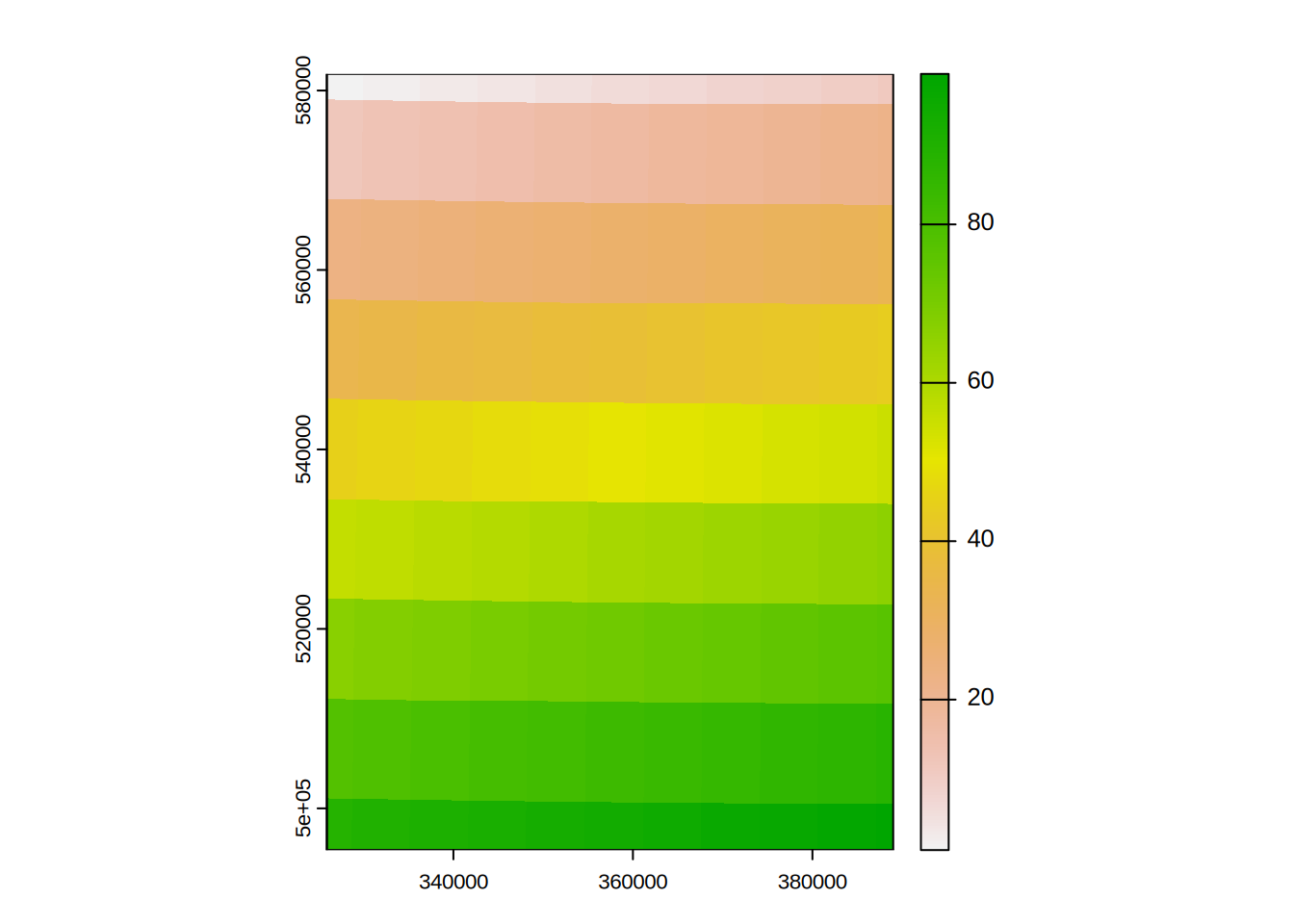
## save
writeRaster(reproj_rid,file.path(".","processed","precip_id.tif"),overwrite=TRUE)
Potential Evapotranspriation
If available spatial Potential Evapotranspiration time series can be
handled in exactly the same way as the rainfall. However if there is
only a single series generatation of the map of id values can be
avoided. A simple sinusoidal PET series can be generated using the
evap_est function in dynatop.
## use a maximum of 3 mm/day - output in meters
pet <- evap_est(index(flow), eMin = 0, eMax = 0.003)
names(pet) <- "pet" # ensure series has a name
Combining Series
The xts package has a convient functions for merging xts objects by the time. We will save this as an R object for later use
obs <- merge(flow,resampled_precip,pet,all=FALSE) ## merge by time stamp
saveRDS(obs,file.path(".","processed","obs.rds"))
WARNING dynatop does not allow for missing data. Any missing values must be replaced during the pre-processing