Altering dynatop
Aim
To a small but substantial change to the dynatop code and rebuild the package
Proposed Change
In this section we will make a change to dynatop by allowing for a different representation in the Hill slope HRU. The new representation of the Hill slope HRU will use and existing transmissivity profile but will treat the potential evapotranspiration as being limited only be the amount of water in the root zone.
This is achieved by
- Altering the R code to allow for an extra value (“bounded_exponential_pet”) to be accepted for the transmissivity value in the options vector of the model
- Developing C++ code for the new implementation
Revised Root Zone Solution
Following the description and notation in the dynatop vignette the revised root zone gains water from precipitation (\(p\)) and the surface zone \(\bar{r}_{sf\rightarrow rz}\). It loses water through evapotranspiration (\(a_p\)) and to the unsaturated zone (\(\bar{r}_{rz \rightarrow uz}\)). Since all the vertical fluxes are spatially uniform the evolution can be evaluated in terms of the spatial averages. The root zone storage satisfies
\[\begin{equation} 0 \leq \bar{s}_{rz} \leq s_{rzmax} \end{equation}\]
with the governing ODE \[\begin{equation} \frac{d\bar{s}_{rz}}{dt} = p - a_p + \bar{r}_{sf\rightarrow rz} - \bar{r}_{rz \rightarrow uz} \end{equation}\]
The rate of evapotranspiration \(a_p\) equally the potential rate \(e_p\) unless \(s_{rz}= 0\) when \[\begin{equation} a_p = \min\left(e_p, p + \bar{r}_{sf\rightarrow rz} - \bar{r}_{rz \rightarrow uz}\right) \end{equation}\]
Fluxes from the surface and to the unsaturated zone are controlled by the level of root zone storage along with the state of the unsaturated and saturated zones.
For \(\bar{s}_{rz} \leq s_{rzmax}\) then \(\bar{r}_{rz \rightarrow uz} \leq 0\). Negative values of \(\bar{r}_{rz \rightarrow uz}\) may occur only when water is returned from the unsaturated zone due to saturation caused by lateral inflow to the saturated zone.
When \(\bar{s}_{rz} = s_{rzmax}\) then \[\begin{equation} p - e_p + \bar{r}_{sf\rightarrow rz} - \bar{r}_{rz \rightarrow uz} \leq 0 \end{equation}\] In this case \(\bar{r}_{rz \rightarrow uz}\) may be positive if \[\begin{equation} p - e_p + \bar{r}_{sf\rightarrow rz} > 0 \end{equation}\] so long as the unsaturated zone can receive the water. If \(\bar{r}_{rz \rightarrow uz}\) is ‘throttled’ by the rate at which the unsaturated zone can receive water, then \(\bar{r}_{sf\rightarrow rz}\) is adjusted (potentially becoming negative) to ensure the equality is met.
Algorithm
Working through the solution an implementation of the approximating equations which is consistent with maximising the downward flux involves an additional step. Following the existing algorithm which makes use of the psuedo-function \(f\left(\check{s}_{sz},\check{r}_{rz \rightarrow uz}\right)\) which returns the value \[\begin{equation} \check{s}_{sz} - \left. \bar{s}_{sz}\right.\rvert_{\Delta 0} - \Delta t \left( \frac{w^{+}}{A}g\left(\check{s}_{sz},\Theta_{sz}\right) - \frac{q_{sz}^{-}}{A} - \min\left(\frac{1}{T_d}, \frac{ \left. \bar{s}_{uz} \right.\rvert_{0} + \Delta t \check{r}_{rz \rightarrow uz} } { T_{d} \check{s}_{sz} + \Delta t} \right) \right) \end{equation}\]
based in part on the transmissivity function \(g\) the new algorithm is given by the following steps:
- Compute \(\check{r}_{sf \rightarrow rz} = \min\left( k_{sf}, \left. \bar{s}_{sf} \right\rvert_{0} + \frac{\Delta t \hat{q}_{sf}^{-}}{A} \right)\)
- Compute \(\check{r}_{rz \rightarrow uz} = \max\left(0, \frac{1}{\Delta t}\left( \left. \bar{s}_{rz} \right.\rvert_{0} + \Delta t \left( p + \check{r}_{sf \rightarrow rz} - e_{p} \right) - s_{rzmax} \right)\right)\)
- Test for saturation. If \(f\left(0,\check{r}_{rz \rightarrow uz}\right) \geq 0\) then goto 4 else goto 5
- Saturated. Set \(\left. \bar{s}_{sz}\right.\rvert_{\Delta t} = 0\) and \(\hat{r}_{rz \rightarrow uz} = \frac{1}{\Delta t}\left( \left. \bar{s}_{sz}\right.\rvert_{0} + \Delta t \left( \frac{w^{+}}{A}g\left(0,\Theta_{sz}\right) - \frac{q_{sz}^{-}}{A}\right) - \left. \bar{s}_{uz} \right.\rvert_{0} \right)\), Goto 7
- Not saturated: find \(\left. \bar{s}_{sz}\right.\rvert_{\Delta t}\) such that \(f\left(\left. \bar{s}_{sz}\right.\rvert_{\Delta t},\check{r}_{rz \rightarrow uz}\right) = 0\).
- Set \(\hat{r}_{rz \rightarrow uz} = \min\left(\check{r}_{rz \rightarrow uz},\frac{1}{\Delta t} \left( \left. \bar{s}_{sz} \right.\rvert_{\Delta t} + \frac{\Delta t}{T_d} - \left. \bar{s}_{uz} \right.\rvert_{0}\right)\right)\).
- Compute the evapotranspiration \(\hat{a}_p = \min\left(e_p, \frac{1}{\Delta t}\left( \left. \bar{s}_{rz}\right.\rvert_{0} + \Delta t \left(p + \check{r}_{sf \rightarrow rz} - \hat{r}_{rz \rightarrow uz}\right)\right)\right)\).
- Compute \(\hat{r}_{sf \rightarrow rz} = \min\left(\check{r}_{sf \rightarrow rz}, \frac{1}{\Delta t}\left( s_{rzmax} - \left. \bar{s}_{rz} \right.\rvert_{0} - \Delta t \left( p - \hat{a}_p - \hat{r}_{rz \rightarrow uz} \right) \right)\right)\)
- Solve for \(\left. \bar{s}_{uz}\right.\rvert_{\Delta t}\), \(\left. \bar{s}_{rz}\right.\rvert_{\Delta t}\) and \(\left. \bar{s}_{sf}\right.\rvert_{\Delta t}\) using the computed vertical fluxes and \(hat{a}_{p}\)
The first two steps compute the maximum potential downward flux from the surface and root zones. Steps 3-6 solve saturated zone and adjust the flux from the root zone to the unsaturated zone accordingly. Step 7 adjusts the evapotranspiration to ensure the root zone storage is not negative. Step 9 adjusts the flux from the surface zone in the case of upward flow from the unsaturated zone, with Step 9 using the corrected vertical fluxes to solve for the new values of the states.
Altering the R code
The key R code in the file dynatop.R. This file contains the code generating the R6 class dyantop and it associated methods (e.g. add_data, sim). Opening the file shows function broken into two groups: public and private. With one exception the public function match the names of the avaialbe methods. The private functions are used by the public functions.
For the for a model with the new option to be accepted in the dynatop code it must first pass the model checks then be used to trigger a call to the correct C++ code.
Checks are performed when the dynatop object is created with
dynatop$new(model). Confusingly this calls the public
initialize function.
From the code in dynatop.R it can be seen that initialize calls in turn two further private functions generate_model_description and check_model.
The function check_model checks the model provided against the description generated by generate_model_description. This means that only this the generation of the model description needs to be changed. The inputs and parameters are identical to those of the “bounded_exponential” transmissivity option, so the changes needed to the generate_model_description function are minimal.
The second set of changes to the R code ensures the correct C++ code
is called. Following the calls from the public initialise and
sim_hillslope functions leads to private functions init_hs and sim_hs.
Both of which contain switch statements which require
alteration.
Adding the C++ code
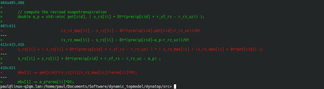
Changing to the handling of the PET input require changes the numerical solution to match the new algorithm. In the src directory copy the file dt_bexp.cpp, the solution to bounded_exponential transmissivity option in the source directory to dt_bexp_pet.cpp. This needs altering to rename the functions to the names used in the R code and to change the algorithm.
The changes can be algorithm are summarised in following the screenshot of a diff between dt_bexp.cpp and dt_bexp_pet.cpp. Line numbers are shown in blue, red and green represent the lines removed and added.
Github repository of waternumbers
Testing
To check the altered code compiled we could use
devtools::check as when building the package. An
alternative way to do it is to use devtools::load_all which
mimics installing then attaching the library.
A test simulation using the model for the Eden catchment build can be done in this way:
devtools::load_all(file.path(".","dynatop")) ## attach the revised package
mdl <- readRDS(file.path(".","processed","atb_band_model.rds")) ## read in the model
obs <- readRDS(file.path(".","processed","obs.rds")) ## read in the observed data
mdl$options["transmissivity_profile"] <- "bounded_exponential_pet" ## change the option
dt <- dynatop$new(mdl) ## create the dynatop object
dt$add_data(obs) ## add the observed data
dt$initialise(obs$Sheepmount_obs[1]/sum(mdl$hillslope$area)) ##initialise the model
dt$sim() ## simulate
mb <- dt$get_mass_errors() ## get the mass balance data
mb$err <- rowSums(mb) ## compute the errors
plot(mb$err) ## plot the errors
Summary
This example has scratched the surface of altering dynatop. To complete the alterations tests should be added, the function documentation altered and the changed algorithm documented in a vignette.
However it demonstrates both the basic structure of the code and the level of complexity required in keeping the numeric solution, input structure and code aligned.