Univariate Gaussian Cost Calculations • anomalous

The purpose of this vignette is to present the calculations of the costs for the univariate Gaussian distribution.

Each time step $t$ belongs to group $k$ whose time stamps are the set $T_{k}$ . A group can have additive mean anomaly $\mu_{k}$ and multiplicative variance anomaly $\sigma_{k}$ which are common for $t \in T_{k}$ . Assuming the {} known mean $m_{t}$ and variance $s_{t}$ of the data generating distribution gives for $t \in T_{k}$

$P\left(y_t \left| m_{t},s_{t}, \mu_k,\sigma_k\right.\right) = \frac{1}{\sqrt{2\pi\sigma_{t}s_{k}}}\exp\left(-\frac{1}{2\sigma_{k}s_{t}}\left(y_{t} - m_t - \mu_{k}\right)^2\right)$

The cost is computed as twice the negative log likelhiood plus a penalty term $\beta$ giving

$C\left(y_{t \in T_{k}} \left| m_{t \in T_{k}}, s_{t \in T_{k}}, \mu_k,\sigma_k\right.\right) = n_{k} \log\left(2\pi \sigma_{k}\right) +\sum\limits_{t \in T_{k}} \log\left(s_{t}\right) +\frac{1}{\sigma_{k}}\sum\limits_{t \in T_{k}} \frac{\left(y_{t} - m_t - \mu_{k}\right)^2}{s_{t}} + \beta$

No Anomaly (Baseline)

Here $\mu_{k}=0$ and $\sigma_{k}=1$ and there is no penalty so the cost is

$C_{B}\left(y_{t \in T_{k}} \left| m_{t \in T_{k}}, s_{t \in T_{k}} \right.\right) = n_{k} \log\left(2\pi \right) +\sum\limits_{t \in T_{k}} \log\left(s_{t}\right) +\sum\limits_{t \in T_{k}} \frac{\left(y_{t} - m_t\right)^2}{s_{t}}$

Collective Anomalies

Collective anomalies last more then a single timestep and chnage the mean and/or variance.

Anomaly in Mean and Variance

Estimates $\hat{\mu}$ of $\mu$ and $\hat{\sigma}$ of $\sigma$ can be selected to minimise the cost by taking

$\hat{\mu}_{k} = \left( \sum\limits_{t \in T_k} \frac{y_t-m_t}{s_t} \right)\left( \sum\limits_{t \in T_k} \frac{1}{s_t}\right)^{-1}$ and $\hat{\sigma}_{k} = \frac{1}{n_{k}} \sum\limits_{t \in T_k} \frac{ \left(y_t-m_t - \hat{\mu}_{k}\right)^2}{s_t}$

Subsituting these into the cost gives $C_{MV}\left(y_{t \in T_{k}} \left| m_{t \in T_{k}}, s_{t \in T_{k}}, \hat{\mu}_k,\hat{\sigma}_k\right.\right) = n_{k} \log\left(2\pi \hat{\sigma}_{k}\right) +\sum\limits_{t \in T_{k}} \log\left(s_{t}\right) +n_{k} + \beta$

Anomaly in Mean

There is no change in variance so $\sigma_{k}=1$ . The Estimate of $\hat{\mu}_{k}$ is unchanged from that for an anomaly in mean and variance so the cost is

$C_{M}\left(y_{t \in T_{k}} \left| m_{t \in T_{k}}, s_{t \in T_{k}}, \hat{\mu}_k\right.\right) = n_{k} \log\left(2\pi\right) +\sum\limits_{t \in T_{k}} \log\left(s_{t}\right) +\sum\limits_{t \in T_k} \frac{ \left(y_t - m_t - \hat{\mu}_{k}\right)^2}{s_t} + \beta$

can be written as

Anomaly in Variance

These is no mean anomaly so $\mu_{k}=0$ . Estimate of $\hat{\sigma}_{k}$ therfore changes to

$\hat{\sigma}_{k} = \frac{1}{n_{k}} \sum\limits_{t \in T_k} \frac{ \left(y_t-m_t\right)^2}{s_t}$

and cost is

$C_{V}\left(y_{t \in T_{k}} \left| m_{t \in T_{k}}, s_{t \in T_{k}}, \hat{\sigma}_k\right.\right) = n_{k} \log\left(2\pi \hat{\sigma}_{k}\right) +\sum\limits_{t \in T_{k}} \log\left(s_{t}\right) +n_{k} + \beta$

Point anomaly

A point anomaly at time $t$ is treated as a single time step with an change in mean or variance. However the cost of the point anomaly should be higher then the background cost when $y_{t}$ is, in some sense, close to the background.

The cost of a point anomaly in mean is expressed as

$C_{P_{M}}\left(y_{t}\left| m_{t},s_{t},\hat{\mu}_{k}\right.\right) = \log\left(2\pi s_{t}\right) + \beta$

while it’s value relative to the baseline cost is can be expressed using the standardised variable $z_{t} = \frac{y_t-m_t}{\sqrt{s_{t}}}$ as

$C_{P_{M}}\left(y_{t}\left| m_{t},s_{t},\hat{\mu}_{k}\right.\right) - C_{B}\left(y_{t}\left| m_{t},s_{t}\right.\right) = \beta - z_{t}^{2}$

The penaly value in this case can then be clearly linked to the number of standard deviations away from the mean at which to declare a point anomaly.

In the case of a point anomaly in variance a naive computation of the cost gives

$C_{P_{V}}\left(y_{t}\left| m_{t},s_{t},\hat{\sigma}_{k}\right.\right)= \log\left(2\pi s_{t} \right) + \log\left(z_{t}^{2}\right) + 1 + \beta$

and

$C_{P_{V}}\left(y_{t}\left| m_{t},s_{t},\hat{\sigma}_{k}\right.\right) - C_{B}\left(y_{t}\left| m_{t},s_{t}\right.\right) = \log\left(z_{t}^{2}\right) + 1 + \beta - z_{t}^2$

Since $\lim\left(z_{t}^{2}\right) \rightarrow \infty$ as $z_{t}^{2} \rightarrow 0$ the niave definition of a point anomaly in variance will always produce point anomalies when $z_{t}$ is close to 0. Fisch et al. introduce a term $\gamma$ to control this. The modified cost of a point anomaly in variance is expressed as

$C_{P_{V}}\left(y_{t}\left| m_{t},s_{t},\hat{\sigma}_{k},\gamma\right.\right)= \log\left(2\pi s_{t} \right) + \log\left(\gamma + z_{t}^{2}\right) + 1 + \beta$

Relating this to the background cost we see that point anomalies may be accepted in the capa search when $f\left(z_{t},\gamma,\beta\right) = C_{P_{V}}\left(y_{t}\left| m_{t},s_{t},\hat{\sigma}_{k},\gamma\right.\right) - C_{B}\left(y_{t}\left| m_{t},s_{t}\right.\right) = \log\left(\gamma + z_{t}^{2}\right) + 1 + \beta - z_{t}^2 < 0$

To ensure that anomalies are not declared when $z_{t}$ is close to 0 this implies that $\gamma$ should be selected such that

$f\left(0,\gamma,\beta\right) \geq 0$
$\gamma < 1$ so the gradient $\frac{\partial}{\partial z_{t}^2} f\left(z_{t},\gamma,\beta\right) = \frac{1}{\gamma + z_{t}^{2}} - 1 > 0$ for $z_{t}$ close to zero.

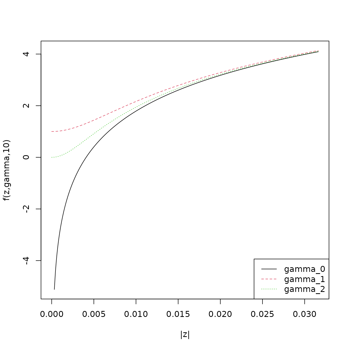
The following plot shows the impact for small $z$ of three different choices of $\gamma$ :

The non correction of $\gamma_{0} = 0$ which allows point anomalies as $z_{t}$ approaches 0
The correction $\gamma_{1} = \exp\left(-\beta\right)$ proposed by Fisch et al.
The minimal correction $\gamma_{2} = \exp\left(-\left(1+\beta\right)\right)$ for which $f\left(0,\gamma_{2},\beta\right) = 0$ .

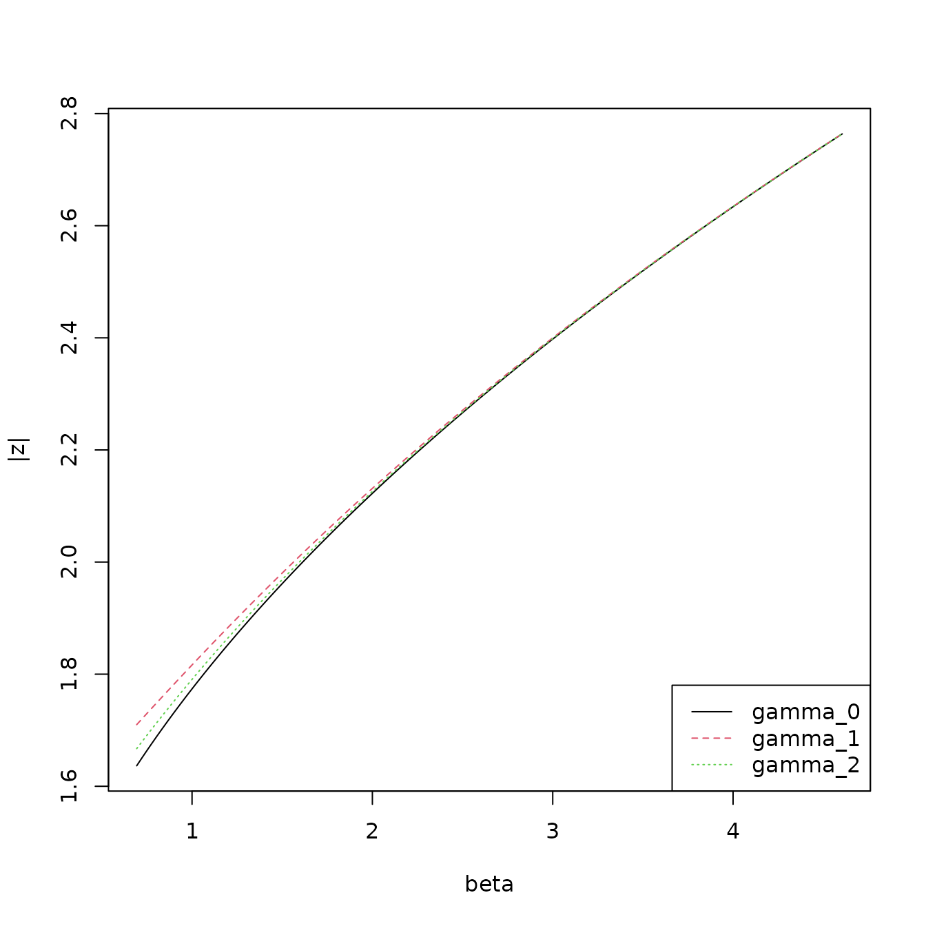
It is clear that the difference become small as $z$ increases. This is supported by the plot below which shows the value of $z_{t}$ at which an point anomaly might occur as $\beta$ varies. Area above the line are potential anomaly values.