Cost Calculations

The purpose of this vignette is to present the calculations of the costs for various distribution.

In the follow variables identified by Greek letters are considered known a priori.

Univariate Independent Gaussian

Data belongs to group $k$ whose time stamps are the set $T_{k}$ can have additive mean anomaly $m_{k}$ and multiplicative variance anomaly $s_{k}$ which are common for $t \in T_{k}$. For $t \in T_{k}$ this gives $$P\left(y_t \left| \mu_t,m_k,\sigma_k,s_k\right.\right) = \frac{1}{\sqrt{2\pi\sigma_{t}s_{k}}}\exp\left(-\frac{1}{2\sigma_{t}s_{k}}\left(y_{t} - \mu_t - m_{k}\right)^2\right)$$

with the likelihood of of the $n_{k}$ observations $y_{t \in T_{k}}$ being $$L\left(y_{t \in T_{k}} \left| \mu_t,m_k,\sigma_k,s_k\right.\right) = \left(2\pi s_{k}\right)^{-n_{k}/2} \prod\limits_{t \in T_{k}} \sigma_{t}^{-1/2} \exp\left(-\frac{1}{2s_{k}}\sum\limits_{t \in T_{k}} \frac{\left(y_{t} - \mu_t - m_{k}\right)^2}{\sigma_{t}}\right)$$

The log-likelihood of $y_{t \in T_{k}}$ is then $$l\left(y_{t \in T_{k}} \left| \mu_t,m_k,\sigma_k,s_k\right.\right) = -\frac{n_{k}}{2} \log\left(2\pi s_{k}\right) -\frac{1}{2}\sum\limits_{t \in T_{k}} \log\left(\sigma_{t}\right) -\frac{1}{2s_{k}}\sum\limits_{t \in T_{k}} \frac{\left(y_{t} - \mu_t - m_{k}\right)^2}{\sigma_{t}}$$

with the cost being twice the negative log likelihood plus a penalty $\beta$ giving

$$C\left(y_{t \in T_{k}} \left| \mu_t,m_k,\sigma_k,s_k\right.\right) = n_{k} \log\left(2\pi s_{k}\right) +\sum\limits_{t \in T_{k}} \log\left(\sigma_{t}\right) +\frac{1}{s_{k}}\sum\limits_{t \in T_{k}} \frac{\left(y_{t} - \mu_t - m_{k}\right)^2}{\sigma_{t}} + \beta$$

Anomaly in mean and varinace

Estimates $\hat{m}$ of $m$ and $\hat{\sigma}$ of $\sigma$ can be selected to minimise the cost by taking $$\hat{m}_{k} = \left( \sum\limits_{t \in T_k} \frac{y_t-\mu_t}{\sigma_t} \right)\left( \sum\limits_{t \in T_k} \frac{1}{\sigma_t}\right)^{-1}$$ and $$\hat{s}_{k} = \frac{1}{n_{k}} \sum\limits_{t \in T_k} \frac{ \left(y_t-\mu_t - \hat{m}_{k}\right)^2}{\sigma_t}$$

Subsituting these into the cost gives $$C_{MV}\left(y_{t \in T_{k}} \left| \mu_t,\hat{m}_k,\sigma_k,\hat{s}_k\right.\right) = n_{k} \log\left(2\pi \hat{s}_{k}\right) +\sum\limits_{t \in T_{k}} \log\left(\sigma_{t}\right) +n_{k} + \beta$$

Anomaly in Mean

There is no change in variance so $s_{k}=1$. Estimate of $\hat{m}_{k}$ is unchanged from that for an anomaly in mean and variance so the cost

$$C_{M}\left(y_{t \in T_{k}} \left| \mu_t,\hat{m}_k,\sigma_k\right.\right) = n_{k} \log\left(2\pi\right) +\sum\limits_{t \in T_{k}} \log\left(\sigma_{t}\right) +\sum\limits_{t \in T_k} \frac{ \left(y_t-\mu_t - \hat{m}_{k}\right)^2}{\sigma_t} + \beta$$

can be written as

$$C_{M}\left(y_{t \in T_{k}} \left| \mu_t,\hat{m}_k,\sigma_k\right.\right) = n_{k} \log\left(2\pi\right) +\sum\limits_{t \in T_{k}} \log\left(\sigma_{t}\right) +\sum\limits_{t \in T_k} \frac{ \left(y_t-\mu_t\right)^2}{\sigma_t} -\hat{m}^{2} \sum\limits_{t \in T_k} \frac{ 1}{\sigma_t} + \beta$$

Anomaly in Variance

These is no mean anomaly so $m_{k}=0$. Estimate of $\hat{s}_{k}$ therfore changes to

$$\hat{s}_{k} = \frac{1}{n_{k}} \sum\limits_{t \in T_k} \frac{ \left(y_t-\mu_t\right)^2}{\sigma_t}$$ and cost is $$C_{V}\left(y_{t \in T_{k}} \left| \mu_t,\sigma_k,\hat{s}_k\right.\right) = n_{k} \log\left(2\pi \hat{s}_{k}\right) +\sum\limits_{t \in T_{k}} \log\left(\sigma_{t}\right) +n_{k} + \beta$$

No Anomaly (Baseline)

Here $m_{k}=0$ and $s_{k}=1$ and there is no penalty so

$$C_{B}\left(y_{t \in T_{k}} \left| \mu_t,\sigma_t\right.\right) = n_{k} \log\left(2\pi \right) +\sum\limits_{t \in T_{k}} \log\left(\sigma_{t}\right) +\sum\limits_{t \in T_{k}} \frac{\left(y_{t} - \mu_t\right)^2}{\sigma_{t}}$$

Point anomaly

A point anomaly at time $t$ is treated as a sinle time step with a variance anomaly. Naively the cost could be computed using the formulea for a variance anomaly as $$C_{p}\left(y_{t}\left| \mu_{t},\sigma_{t}\right.\right) = \log\left(2\pi \frac{ \left(y_t-\mu_t\right)^2}{\sigma_t}\right) + \log\left(\sigma_{t}\right) + 1 + \beta = \log\left(2\pi\right) + \log \left( \left(y_t-\mu_t\right)^2 \right) + 1 + \beta$$

However the cost of the point anomaly should be higher then the background cost when $y_{t}$ is, in some sense, close to the background.

Follow Fisch et al. in intorducing a term $\gamma$ to control this. Using the standardised variable $z_{t} = \frac{y_t-\mu_t}{\sqrt{\sigma_{t}}}$ the modified cost of a point anomaly is expressed as $$C_{p}\left(y_{t}\left| \mu_{t},\sigma_{t}\right.\right) = \log\left(2\pi\right) + \log\left(\sigma_{t}\right) + \log \left( \gamma + z_{t}^{2} \right) + 1 + \beta$$

Relating this to the background cost we see that point anomalies may be accepted in the capa search when $$f\left(z_{t}^2,\gamma,\beta\right) = C_{p}\left(y_{t}\left| \mu_{t},\sigma_{t}\right.\right) - C_{B}\left(y_{t}\left| \mu_{t},\sigma_{t}\right.\right) = \log \left( \gamma + z_{t}^{2} \right) + 1 + \beta - z_{t}^{2} < 0$$

This implies that $\gamma$ should be selected such that $f\left(0,\gamma,\beta\right) \geq 0$

The gradient wrt $z_{t}^2$ is $$\frac{\partial}{\partial z_{t}^2} f\left(z_{t}^2,\gamma,\beta\right) = \frac{1}{\gamma + z_{t}^{2}} - 1$$

Requiring $\gamma < 1$; which maintains a positive gradient for small z_{t}^2; indicates that there will no anomalies near 0.

Consider three different definitions of $\gamma$.

• The non corection of $\gamma_{0} = 0$ which allows point anomalies as z_{t}^2 approaches 0
• The correction $\gamma_{1} = \exp\left(-\beta\right)$ proposed by Fisch et al.
• The minimal correction $\gamma_{2} = \exp\left(-\left(1+\beta\right)\right)$ for which $f\left(0,\gamma_{2},\beta\right) = 0$.

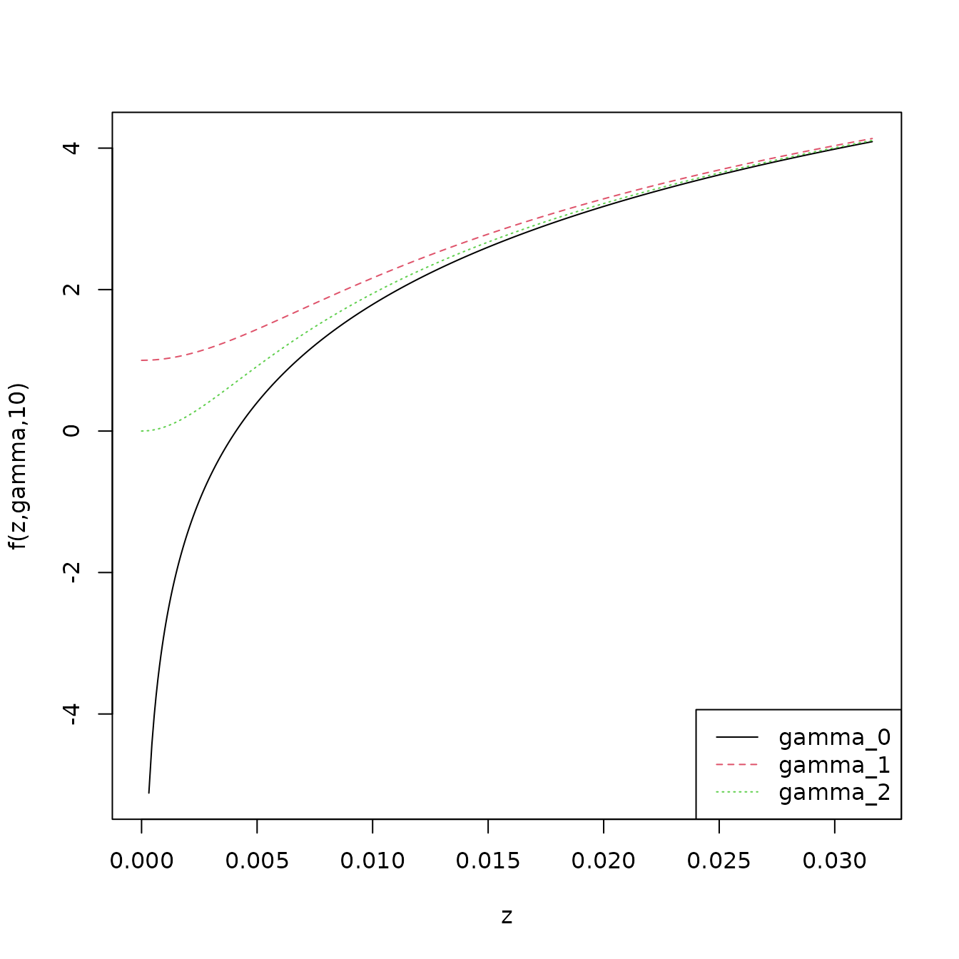
To see the impact of the correct for small $z$ the following figure shows $f\left(z_{t}^2,\gamma,\beta\right)$ for $\beta=10$ for the three options.

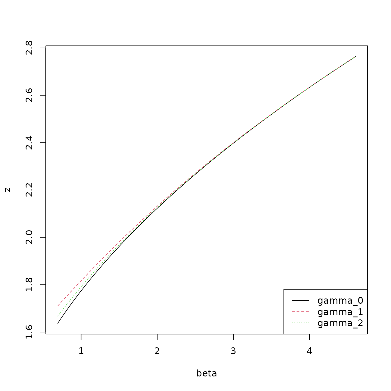
It is clear that the difference become small as $z$ increases. This is supported by the plot below shows the value of $z_{t}$ at which an point anomaly might occur as $\beta$ varies. Area above the line are potential anomaly values.

Poisson

Data belongs to group $k$ whose time stamps are the set $T_{k}$ can have a multiplicative rate anomaly $r_{k}$ which is common for $t \in T_{k}$. For $t \in T_{k}$ this gives $$P\left(y_t \left| \lambda_t,r_k\right.\right) = \frac{\lambda_{t}^{y_{t}} r_{k}^{y_{t}} \exp\left(-r_{k}\lambda_{t}\right)}{y_{t}!}$$

with the likelihood of of the $n_{k}$ observations $y_{t \in T_{k}}$ being $$L\left(y_{t \in T_{k}} \left| \lambda_t,r_k\right.\right) = r_{k}^{\sum\limits_{t \in T_{k}} y_{t}} \exp\left(-r_{k} \sum\limits_{t \in T_{k}} \lambda_{t}\right) \prod\limits_{t \in T_{k}} \frac{ \lambda_{t}^{y_{t}} }{ y_{t}!}$$

The log-likelihood of $y_{t \in T_{k}}$ is then $$l\left(y_{t \in T_{k}} \left| \lambda_t,r_k\right.\right) = \sum\limits_{t \in T_{k}} y_{t} \log\left(r_{k}\right) - r_{k} \sum\limits_{t \in T_{k}} \lambda_{t} + \sum\limits_{t \in T_{k}} y_{t} \log\left(\lambda_{t}\right) - \sum\limits_{t \in T_{k}} \log\left( y_{t}! \right)$$

with the cost being twice the negative log likelihood plus a penalty $\beta$ giving

$$C\left(y_{t \in T_{k}} \left| \lambda_t,r_k\right.\right) = 2 r_{k} \sum\limits_{t \in T_{k}} \lambda_{t} - 2 \sum\limits_{t \in T_{k}} y_{t} \log\left(r_{k}\right) - 2 \sum\limits_{t \in T_{k}} y_{t} \log\left(\lambda_{t}\right) + 2 \sum\limits_{t \in T_{k}} \log\left( y_{t}! \right) +\beta$$

Anomaly in rate

Estimates $\hat{r}_{k}$ of $r_{k}$ can be selected to minimise the cost by taking $$\hat{r}_{k} = \frac{ \sum\limits_{t \in T_{k}} y_{t} }{\sum\limits_{t \in T_{k}} \lambda_{t}}$$

This gives a cost of $$C\left(y_{t \in T_{k}} \left| \lambda_t,r_k\right.\right) = 2 \sum\limits_{t \in T_{k}} y_{t} - 2 \sum\limits_{t \in T_{k}} y_{t} \log\left(\hat{r}_{k}\right) - 2 \sum\limits_{t \in T_{k}} y_{t} \log\left(\lambda_{t}\right) + 2 \sum\limits_{t \in T_{k}} \log\left( y_{t}! \right) + \beta$$

No Anomaly (Baseline)

Here $r_{k}=1$ and there is no penalty so

$$C_{B}\left(y_{t \in T_{k}} \left| \lambda_t,r_k\right.\right) = 2 \sum\limits_{t \in T_{k}} \lambda_{t} - 2 \sum\limits_{t \in T_{k}} y_{t} \log\left(\lambda_{t}\right) + 2 \sum\limits_{t \in T_{k}} \log\left( y_{t}! \right)$$

Point anomaly

A point anomaly at time $t$ is treated as a single time step rate anomaly. Naively the cost could be computed using the formulea for a rate anomaly with $\hat{r}_{k} = y_{t}/\lambda_{t}$ giving

$$C_{P}\left(y_{t} \left| \lambda_t,r_k\right.\right) = 2 y_{t} - 2 y_{t} \log\left(y_{k}\right) + 2 \log\left( y_{t}! \right) + \beta$$

However the cost of the point anomaly should be higher then the background cost when $r_{k}$ is, in some sense, close to the background value of 1.

Comparing to the baseline cost for a single point shows that a point anomaly will exist when

$$2 y_{t} - 2 y_{t} \log\left(y_{k}\right) + 2 \log\left( y_{t}! \right) + \beta < 2 \lambda_{t} - 2 y_{t} \log\left(\lambda_{t}\right) + 2 \log\left( y_{t}! \right)$$

Rearrangement gives

$$\begin{equation} \beta < 2 \left( \lambda_{t} - y_{t} \right) + 2 y_{t} \left( \log\left(y_{t}\right) - \log\left(\lambda_{t}\right) \right) \\ < 2 \lambda_{t} \left( 1 - r_{k} \right) + 2 y_{t} \log\left(r_{k}\right) \\ < 2 \lambda_{t} \left( 1 - r_{k} + r_{k} \log\left(r_{k}\right) \right) \end{equation}$$

The follwoing plot shows that selection of $\beta$ can be selected as a multiple of $\lambda$ to avoid $r$ being to close to 1.

Multivariate Gaussian

A vector of data $\mathbf{y}$ of length $p$ follows a multivariate Gaussian with mean $\mathbf{\mu}$ and precision $\mathbf{\Lambda}$.

Background

Without any anomalous periods the log liklihood is given by

$$l\left(\mathbf{y}\left| \mathbf{\mu}, \mathbf{\Lambda} \right. \right) = -\frac{p}{2}\log\left(2\pi\right) - \frac{1}{2}\log\left|\mathbf{\Lambda}^{-1}\right| - \frac{1}{2} \left(\mathbf{y}-\mathbf{\mu}\right)^{T} \mathbf{\Lambda} \left(\mathbf{y}-\mathbf{\mu}\right)$$

or as a cost

$$C\left(\mathbf{y}\left| \mathbf{\mu}, \mathbf{\Sigma} \right. \right) = p\log\left(2\pi\right) - \log\left|\mathbf{\Lambda}\right| + \left(\mathbf{y}-\mathbf{\mu}\right)^{T} \mathbf{\Lambda} \left(\mathbf{y}-\mathbf{\mu}\right)$$

Modelling anomalies

Consider the $i$th of $K$ anomalies occurs of consecuative time steps starting at time $s^\left[i\right]$ and finished at $e^\left[i\right]$. Anomalies do not overlap so $e^\left[i\right] < s^\left[j\right]$ for all $0<i<j<K$

To model change in variance let $\Omega$ be a $p \times p$ diagonal matrix where $\Omega_{t,t} = \omega^{\left[i\right]}$ if there exists $i$ such that $s^\left[i\right] \leq t \leq e^\left[i\right]$ and 1 otherwise.

Let $\delta$ be a length $K$ vector of mean changes and $\mathbf{X}$ a $p \times K$ matrix where $\mathbf{X}_{t,i}=1$ if $s^\left[i\right] \leq t \leq e^\left[i\right]$ and zero otherwise.

Decomposing $\Lambda$ such that $\mathbf{\Lambda} = \mathbf{U}^{T}\mathbf{U}$ the costs including anomalies becomes

$$C\left(\mathbf{y}\left| \mathbf{\mu}, \mathbf{\Sigma}, \delta, \Omega \right. \right) = p\log\left(2\pi\right) - \log\left| \mathbf{U}^{T}\Omega\mathbf{U} \right| + \left(\mathbf{y}-\mathbf{\mu}-\mathbf{X}\delta\right)^{T} \mathbf{U}^{T}\Omega\mathbf{U} \left(\mathbf{y}-\mathbf{\mu}-\mathbf{X}\delta\right)$$

Solving for $\omega$ and $\delta$

Let $\mathbf{d} = \mathbf{U}\left(\mathbf{y}=\mu\right)$ and $\mathbf{D} = \mathbf{U} \mathbf{X}$. Using this the cost is $$C\left(\mathbf{y}\left| \mathbf{\mu}, \mathbf{\Sigma}, \delta, \Omega \right. \right) = p\log\left(2\pi\right) - \log\left| \mathbf{U}^{T}\Omega\mathbf{U} \right| + \left(\mathbf{d} - \mathbf{D}\delta\right)^{T} \Omega \left(\mathbf{d} - \mathbf{D}\delta\right)$$

Since $\Omega$ is diagonal $$\left(\mathbf{d} - \mathbf{D}\delta\right)^{T} \Omega \left(\mathbf{d} - \mathbf{D}\delta\right) = \sum\limits_{t=1:p} \Omega_{t,t}\left(\mathbf{d}_{t} - \mathbf{D}_{t,.}\delta\right)^{2}$$

For an non-anoalous time step $t \in T^{\prime}$ we see that $\Omega_{t,t}=1$ and $\mathbf{D}_{t,.}=\mathbf{0}$ allowing the summation to be written $$\sum\limits_{t=1:p} \Omega_{t,t}\left(\mathbf{d}_{t} - \mathbf{D}_{t,.}\delta\right)^{2}= \sum\limits_{t \in T^{\prime}} \mathbf{d}_{t}^{2} + \sum\limits_{k=1:K} \omega_{k} \sum\limits_{t=s^{\left[k\right]}:e^{\left[k\right]}} \left(\mathbf{d}_{t} - \mathbf{D}_{t,.}\delta\right)^{2}$$

Using the identities for determinants gives $$\log\left| \mathbf{U}^{T}\Omega\mathbf{U} \right| = \log\left| \mathbf{U}^{T}\mathbf{U} \right| + \log\left| \Omega \right|$$ and $$\log\left| \Omega \right| = \sum\limits_{k=1:K} \left(s^{\left[k\right]}-e^{\left[k\right]}+1\right) \log \omega_{k}$$

Subsituation of these terms into the cost function gives $$\frac{\partial}{\partial \omega_{k}} C\left(\mathbf{y}\left| \mathbf{\mu}, \mathbf{\Sigma}, \delta, \Omega \right. \right) = - \frac{\left(s^{\left[k\right]}-e^{\left[k\right]}+1\right)}{\omega_{k}} + \sum\limits_{t=s^{\left[k\right]}:e^{\left[k\right]}} \left(\mathbf{d}_{t} - \mathbf{D}_{t,.}\delta\right)^{2}$$