Plotting fks objects

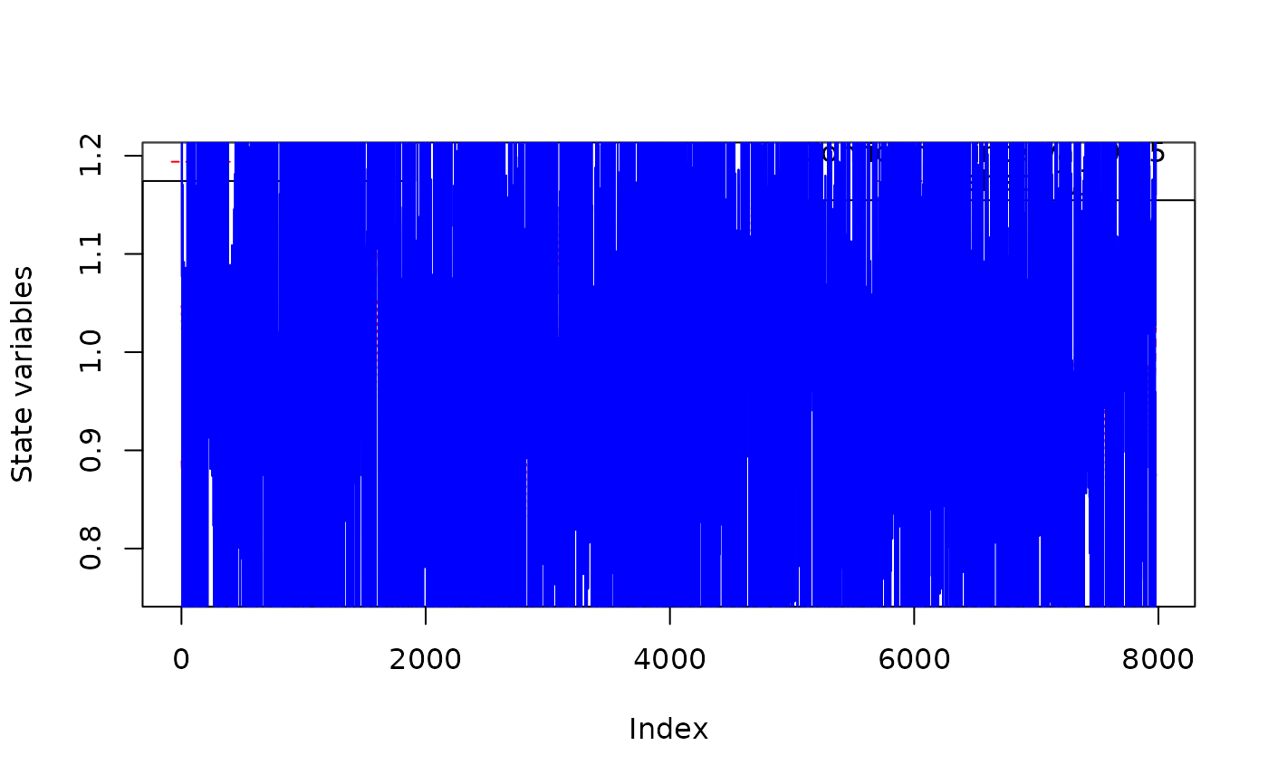
Plotting method for objects of class fks. This function provides tools visualisation of the state vector of the Kalman smoother output

# S3 method for class 'fks'
plot(x, CI = 0.95, ahatt.idx = 1:nrow(x$ahatt), ...)

Arguments

x

The output of fks.

CI

The confidence interval in case type == "state". Set CI to NA if no confidence interval shall be plotted.

ahatt.idx

An vector giving the indexes of the predicted state variables which shall be plotted if type == "state".

...

Arguments passed to either plot, qqnorm, qqplot or acf.

Details

The state variables are plotted. By the argument ahatt.idx, the user can specify which of the smoothed (\(a_{t|n}\)) state variables will be drawn.

See also

fks

Examples

## <--------------------------------------------------------------------------->
## Example 3: Local level model for the treering data
## <--------------------------------------------------------------------------->
## Transition equation:
## alpha[t+1] = alpha[t] + eta[t], eta[t] ~ N(0, HHt)          
## Measurement equation:
## y[t] = alpha[t] + eps[t], eps[t] ~  N(0, GGt)

y <- treering
y[c(3, 10)] <- NA  # NA values can be handled

## Set constant parameters:
dt <- ct <- matrix(0)
Zt <- Tt <- array(1,c(1,1,1))
a0 <- y[1]            # Estimation of the first width
P0 <- matrix(100)     # Variance of 'a0'

## Estimate parameters:
fit.fkf <- optim(c(HHt = var(y, na.rm = TRUE) * .5,
                   GGt = var(y, na.rm = TRUE) * .5),
                 fn = function(par, ...)
                 -fkf(HHt = array(par[1],c(1,1,1)), GGt = array(par[2],c(1,1,1)), ...)$logLik,
                 yt = rbind(y), a0 = a0, P0 = P0, dt = dt, ct = ct,
                 Zt = Zt, Tt = Tt)

## Filter tree ring data with estimated parameters:
fkf.obj <- fkf(a0, P0, dt, ct, Tt, Zt, HHt = array(fit.fkf$par[1],c(1,1,1)),
               GGt = array(fit.fkf$par[2],c(1,1,1)), yt = rbind(y))

fks.obj <- fks(fkf.obj)
plot(fks.obj)

##lines(as.numeric(y),col="blue")