To demonstrate the use of the FKF package this example
shows how to fit an ARMA(2, 1) model using this Kalman filter
implimentation and teh extraction of the resulting filtered and smoothed
estimates.
Start by loading the package:
Estimation
To estimate the parameters using numerical optimisation two functions are specified. The first creates a state space representation out of the four ARMA parameters
arma21ss <- function(ar1, ar2, ma1, sigma) {
    Tt <- matrix(c(ar1, ar2, 1, 0), ncol = 2)
    Zt <- matrix(c(1, 0), ncol = 2)
    ct <- matrix(0)
    dt <- matrix(0, nrow = 2)
    GGt <- matrix(0)
    H <- matrix(c(1, ma1), nrow = 2) * sigma
    HHt <- H %*% t(H)
    a0 <- c(0, 0)
    P0 <- matrix(1e6, nrow = 2, ncol = 2)
    return(list(a0 = a0, P0 = P0, ct = ct, dt = dt, Zt = Zt, Tt = Tt, GGt = GGt,
                HHt = HHt))
}
The second is the objective function passed to optim
which returns the noegative log-likelihood
objective <- function(theta, yt) {
    sp <- arma21ss(theta["ar1"], theta["ar2"], theta["ma1"], theta["sigma"])
    ans <- fkf(a0 = sp$a0, P0 = sp$P0, dt = sp$dt, ct = sp$ct, Tt = sp$Tt,
               Zt = sp$Zt, HHt = sp$HHt, GGt = sp$GGt, yt = yt)
    return(-ans$logLik)
}
Estimation is then performed using a numeric search by
optim
Results
First consider the 95% CI for the parameter estimate which can be constructed using the hessian of the fit:
## Confidence intervals
p <- cbind(actual = c(ar1=ar1,ar2=ar2,ma1=ma1,sigma=sigma),
           estimate = fit$par,
           lowerCI = fit$par - qnorm(0.975) * sqrt(diag(solve(fit$hessian))),
           upperCI = fit$par + qnorm(0.975) * sqrt(diag(solve(fit$hessian))))
p
#>          actual    estimate    lowerCI   upperCI
#> ar1    0.600000  0.44220027  0.2483370 0.6360635
#> ar2    0.200000  0.27865796  0.1527385 0.4045774
#> ma1   -0.200000 -0.01510979 -0.2157122 0.1854926
#> sigma  1.414214  1.41943609  1.3571952 1.4816770
showing the actual parameters fall within the 95% CI of the estimated values.
The series can be filtered using the estimated parameter values
sp <- arma21ss(fit$par["ar1"], fit$par["ar2"], fit$par["ma1"], fit$par["sigma"])
ans <- fkf(a0 = sp$a0, P0 = sp$P0, dt = sp$dt, ct = sp$ct, Tt = sp$Tt,
           Zt = sp$Zt, HHt = sp$HHt, GGt = sp$GGt, yt = rbind(a))
This allows comparision of the prediction with the realization
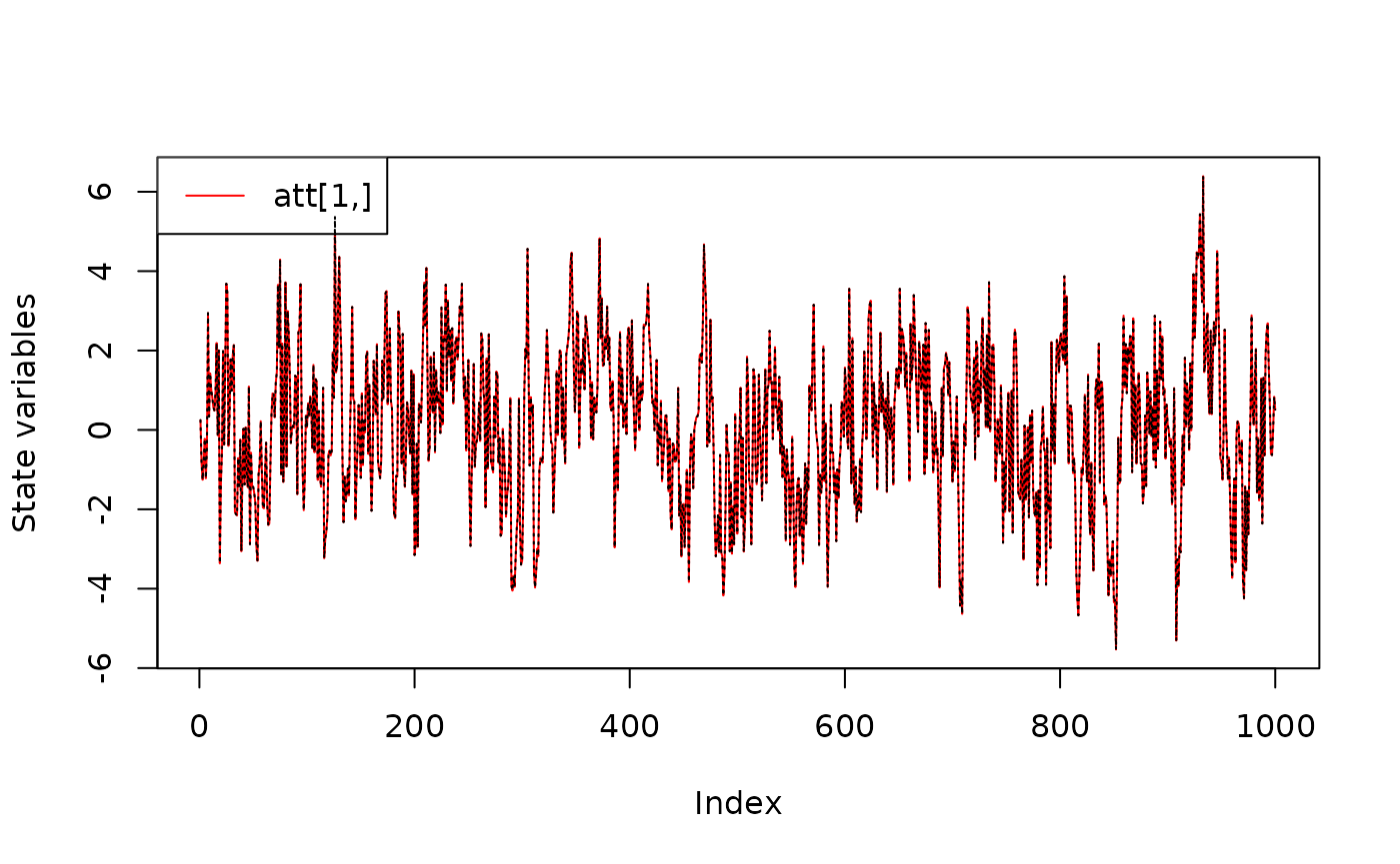
 and comparision of the filtered series with the realization

The plotting function for the fkf class also allows visual checking of whether the residuals are Gaussian
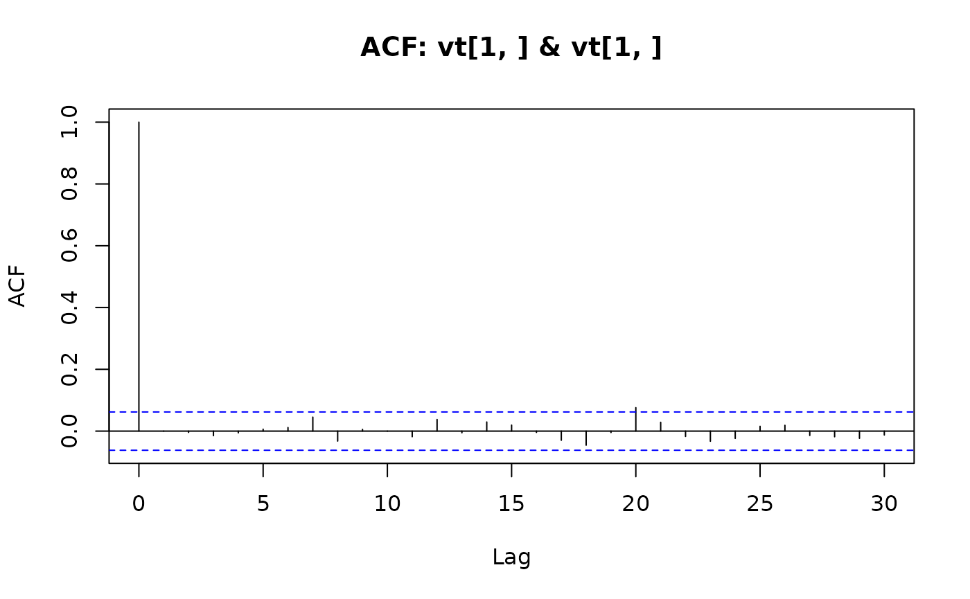
plot(ans, type = "resid.qq") or if there is a linear serial dependence through ‘acf’
plot(ans, type = "acf")
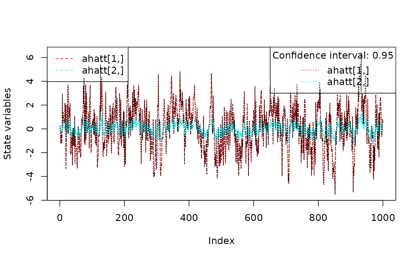
The smoothed estimates can also be computed by a simple call to fks
sm <- fks(ans)The smoothed estiamte with confidence intervals can be plotted alongside the observed data
