Plotting fkf objects

Plotting method for objects of class fkf. This function provides tools for graphical analysis of the Kalman filter output: Visualization of the state vector, QQ-plot of the individual residuals, QQ-plot of the Mahalanobis distance, auto- as well as crosscorrelation function of the residuals.

# S3 method for class 'fkf'
plot(
  x,
  type = c("state", "resid.qq", "qqchisq", "acf"),
  CI = 0.95,
  at.idx = 1:nrow(x$at),
  att.idx = 1:nrow(x$att),
  ...
)

Arguments

x: The output of fkf.
type: A string stating what shall be plotted (see Details).
CI: The confidence interval in case type == "state". Set CI to NA if no confidence interval shall be plotted.
at.idx: An vector giving the indexes of the predicted state variables which shall be plotted if type == "state".
att.idx: An vector giving the indexes of the filtered state variables which shall be plotted if type == "state".
...: Arguments passed to either plot, qqnorm, qqplot or acf.

Value

Invisibly returns an list with components:

`distance`	The Mahalanobis distance of the residuals as a vector of length $n$.
`std.resid`	The standardized residuals as an $d \times n$-matrix. It should hold that $std.resid_{ij} \; iid \sim N_d(0, I)$,

where $d$ denotes the dimension of the data and $n$ the number of observations.

Details

The argument type states what shall be plotted. type must partially match one of the following:

state: The state variables are plotted. By the arguments at.idx and att.idx, the user can specify which of the predicted ($a_{t}$) and filtered ($a_{t|t}$) state variables will be drawn.
resid.qq: Draws a QQ-plot for each residual-series invt.
qqchisq: A Chi-Squared QQ-plot will be drawn to graphically test for multivariate normality of the residuals based on the Mahalanobis distance.
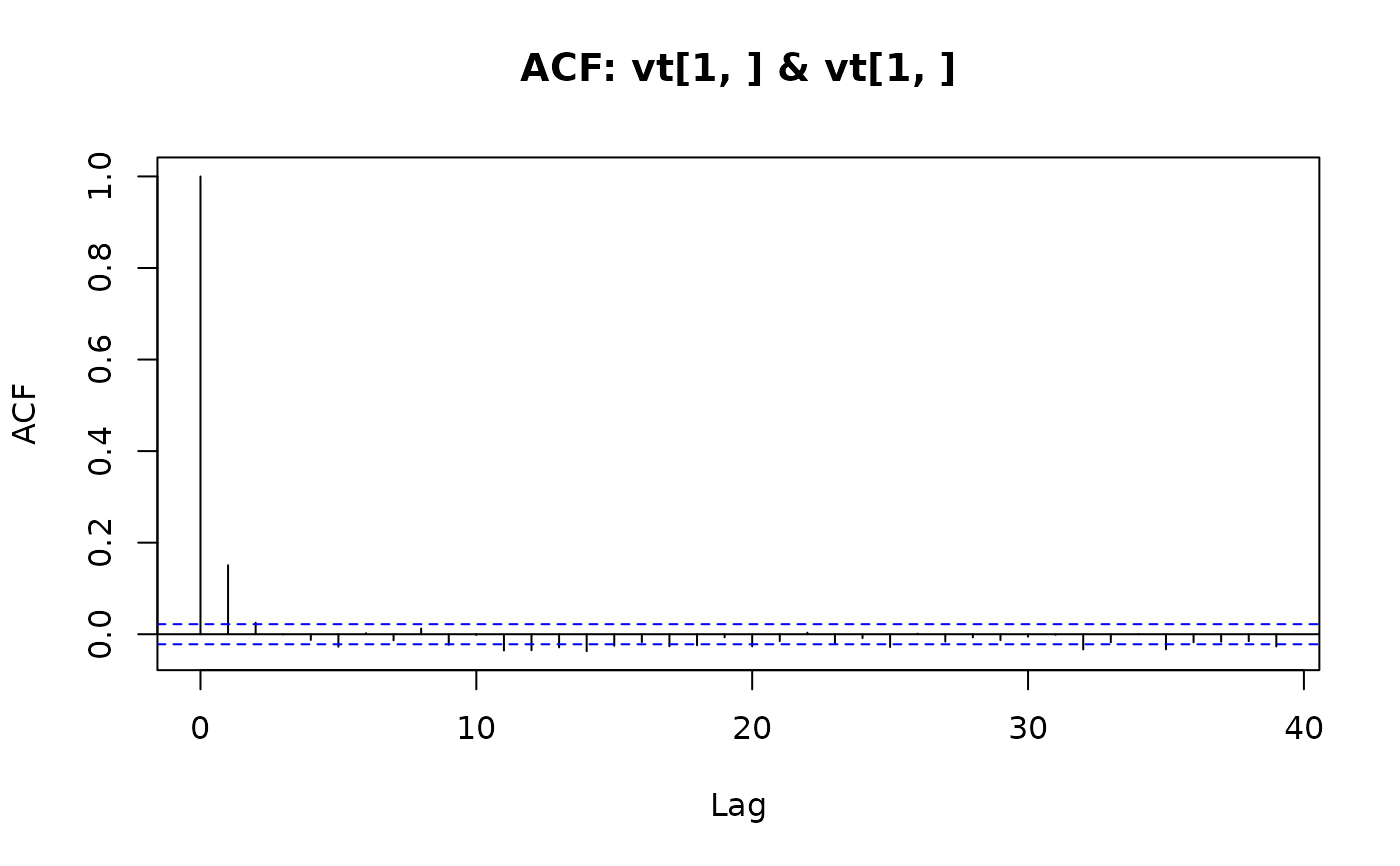
acf: Creates a pairs plot with the autocorrelation function (acf) on the diagonal panels and the crosscorrelation function (ccf) of the residuals on the off-diagnoal panels.

usage

plot(x, type = c("state", "resid.qq", "qqchisq", "acf"), CI = 0.95, at.idx = 1:nrow(x$at), att.idx = 1:nrow(x$att), ...)

Examples

## <--------------------------------------------------------------------------->
## Example: Local level model for the treering data
## <--------------------------------------------------------------------------->
## Transition equation:
## alpha[t+1] = alpha[t] + eta[t], eta[t] ~ N(0, HHt)          
## Measurement equation:
## y[t] = alpha[t] + eps[t], eps[t] ~  N(0, GGt)

y <- treering
y[c(3, 10)] <- NA  # NA values can be handled

## Set constant parameters:
dt <- ct <- matrix(0)
Zt <- Tt <- array(1,c(1,1,1))
a0 <- y[1]            # Estimation of the first width
P0 <- matrix(100)     # Variance of 'a0'

## Estimate parameters:
fit.fkf <- optim(c(HHt = var(y, na.rm = TRUE) * .5,
                   GGt = var(y, na.rm = TRUE) * .5),
                 fn = function(par, ...)
                 -fkf(HHt = array(par[1],c(1,1,1)), GGt = array(par[2],c(1,1,1)), ...)$logLik,
                 yt = rbind(y), a0 = a0, P0 = P0, dt = dt, ct = ct,
                 Zt = Zt, Tt = Tt)

## Filter tree ring data with estimated parameters:
fkf.obj <- fkf(a0, P0, dt, ct, Tt, Zt, HHt = array(fit.fkf$par[1],c(1,1,1)),
               GGt = array(fit.fkf$par[2],c(1,1,1)), yt = rbind(y))

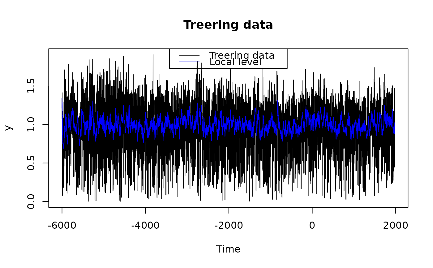
## Plot the width together with fitted local levels:
plot(y, main = "Treering data")
lines(ts(fkf.obj$att[1, ], start = start(y), frequency = frequency(y)), col = "blue")
legend("top", c("Treering data", "Local level"), col = c("black", "blue"), lty = 1)


## Check the residuals for normality:
plot(fkf.obj, type = "resid.qq")


## Test for autocorrelation:
plot(fkf.obj, type = "acf", na.action = na.pass)

Arguments

Value

Details

usage

See also

Examples